Chapter 5 Simulation of Random Variables

In this chapter we discuss simulation related to random variables. After a review of probability simulation, we turn to the estimation of pdfs and pmfs of random variables. These simulations provide a foundation for understanding the fundamental concepts of statistical inference: sampling distributions, point estimators, and the Central Limit Theorem.

5.1 Estimating probabilities

In order to run simulations with random variables, we use R’s built-in random generation functions. These functions all take the form rdistname, where distname is the root name of the distribution. Normal random variables have root norm, so the random generation function for normal rvs is rnorm. Other root names we have encountered so far are unif, geom, pois, exp, and binom.

The first argument to all of R’s random generation functions is always the number of samples to create. Random generation functions take additional parameters that fully describe the distribution. For example, if we want to create a random sample of size 100 from a normal random variable with mean 5 and sd 2, we would use rnorm(100, mean = 5, sd = 2), or simply rnorm(100, 5, 2). Without the additional arguments, rnorm gives the standard normal random variable, with mean 0 and sd 1. For example, rnorm(10000) gives 10,000 independent random values of the standard normal random variable \(Z\).

Our strategy for estimating probabilities of events involving random variables is as follows:

• Sample the random variable using the appropriate random generation function.
• Evaluate the event to get a vector of true/false values.
• Use the mean function to compute the proportion of times that the event occurs.

If the sample size is reasonably large, then the true probability that the event occurs should be close to the percentage of times that the event occurs in our sample. The larger the sample size is, the closer we expect our estimate to be to the true value. In practice, a sample of size 10,000 gives a good balance between speed and accuracy. Estimates vary, and rare events are harder to sample, so you should always repeat your estimate a few times to see what kind of variation you obtain in your answers.

Example 5.1

Let \(Z\) be a standard normal random variable. Estimate \(P(Z > 1)\).

We begin by creating a large random sample from a normal random variable.

Z <- rnorm(10000)
head(Z)

## [1]  0.8826500 -0.5235463 -0.9814831  1.1042537  0.5727897  0.3843779

Next, we evaluate the event \(Z > 1\). We create a vector bigZ that is TRUE when the sample is greater than one, and FALSE when the sample is not greater than one.

bigZ <- Z > 1
head(bigZ)

## [1] FALSE FALSE FALSE  TRUE FALSE FALSE

Now, we count the number of times we see a TRUE, and divide by the length of the vector.

sum(bigZ == TRUE) / 10000

## [1] 0.1588

There are a few improvements we can make. First, bigZ == TRUE is just the same as bigZ, so we can compute:

sum(bigZ) / 10000

## [1] 0.1588

We note that sum converts TRUE to one and FALSE to zero. Adding up those values and dividing by the length is the same thing as taking the mean. So, we can simply do:

mean(bigZ)

## [1] 0.1588

For simple problems like this one, there is no real need to store the event in a variable, so we may go directly to the computation:

mean(Z > 1)

## [1] 0.1588

We estimate that \(P(Z > 1) =\) 0.1588.

Example 5.2

Let \(Z\) be a standard normal rv. Estimate \(P(Z^2 > 1)\).

Z <- rnorm(10000)
mean(Z^2 > 1)

## [1] 0.322

We can also easily estimate means and standard deviations of random variables. To do so, we create a large random sample from the distribution in question, and we take the mean or standard deviation of the large sample. If the sample is large, then we expect the sample mean to be close to the true mean, and the sample standard deviation to be close to the true standard deviation. Let’s begin with an example where we know what the correct answer is, in order to check that the technique is working.

Example 5.3

Let \(Z\) be a normal random variable with mean 0 and standard deviation 1. Estimate the mean and standard deviation of \(Z\).

Z <- rnorm(10000)
mean(Z)

## [1] 0.001501601

sd(Z)

## [1] 1.003491

We see that we are reasonably close to the correct answers of 0 and 1.

Example 5.4

Estimate the mean and standard deviation of \(Z^2\).

Z <- rnorm(10000)
mean(Z^2)

## [1] 0.9873908

sd(Z^2)

## [1] 1.416691

We will see later in this chapter that \(Z^2\) is a \(\chi^2\) random variable with one degree of freedom. It is known that a \(\chi^2\) random variable with \(\nu\) degrees of freedom has mean \(\nu\) and standard deviation \(\sqrt{2\nu}\). Thus, the answers above are pretty close to the correct answers.

Example 5.5

Let \(X\) and \(Y\) be independent standard normal random variables. Estimate \(P(XY > 1)\).

There are two ways to do this. The first is:

X <- rnorm(10000)
Y <- rnorm(10000)
mean(X * Y > 1)

## [1] 0.105

A technique that is closer to what we will be doing below is the following. We want to create a random sample from the random variable \(W = XY\). To do so, we would use

W <- rnorm(10000) * rnorm(10000)

Note that R multiplies the vectors component-wise. Then, we compute the percentage of times that the sample is greater than 1 as before.

mean(W > 1)

## [1] 0.0995

The two methods give slightly different answers because simulations are random and only estimate the true values.

Notice that \(P(XY > 1)\) is not the same as the answer we got for \(P(Z^2 > 1)\) in Example 5.2.

5.2 Estimating discrete distributions

In this section, we show how to estimate the pmf of a discrete random variable via simulation. Let’s begin with an example.

Example 5.6

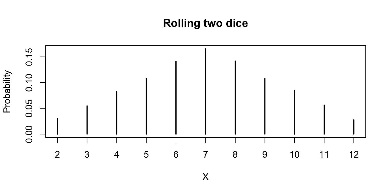
Suppose that two dice are rolled, and their sum is denoted as \(X\). Estimate the pmf of \(X\) via simulation.

To estimate \(P(X = 5)\), for example, we would use

X <- replicate(10000, {
  dieRoll <- sample(1:6, 2, TRUE)
  sum(dieRoll)
})
mean(X == 5)

## [1] 0.1107

It is possible to repeat this approach for each value \(2, 3, \ldots, 12\), but that would take a long time. A more efficient method is to keep track of all observations of the random variable, and divide each by the total number of times the rv was observed. We will use table for this. Recall, table gives a vector of counts of each unique element in a vector. That is,

table(c(1, 1, 1, 1, 1, 2, 2, 3, 5, 1))

## 
## 1 2 3 5 
## 6 2 1 1

indicates that there are 6 occurrences of “1,” 2 occurrences of “2,” and 1 occurrence each of “3” and “5.” To apply this to the die rolling, we create a vector of length 10,000 that has all observations of the random variable \(X\):

X <- replicate(10000, {
  dieRoll <- sample(1:6, 2, TRUE)
  sum(dieRoll)
})
table(X)

## X
##    2    3    4    5    6    7    8    9   10   11   12 
##  300  547  822 1080 1412 1655 1418 1082  846  562  276

We then divide each entry of the table by 10,000 to estimate of the pmf of \(X\):

table(X) / 10000

## X
##      2      3      4      5      6      7      8      9     10     11 
## 0.0300 0.0547 0.0822 0.1080 0.1412 0.1655 0.1418 0.1082 0.0846 0.0562 
##     12 
## 0.0276

We don’t want to hard-code the 10,000 value in the above command, because it can be a source of error if we change the number of replications and forget to change the denominator here. There is a base R function proportions²⁶ which is useful for dealing with tabled data. In particular, if the tabled data is of the form above, then it computes the proportion of each value.

proportions(table(X))

## X
##      2      3      4      5      6      7      8      9     10     11 
## 0.0300 0.0547 0.0822 0.1080 0.1412 0.1655 0.1418 0.1082 0.0846 0.0562 
##     12 
## 0.0276

And, there is our estimate of the pmf of \(X\). For example, we estimate the probability of rolling an 11 to be 0.0562.

A simple way to visualize a pmf is to plot the table:

plot(proportions(table(X)),
  main = "Rolling two dice", ylab = "Probability"
)

Example 5.7

Suppose 50 randomly chosen people are in a room. Let \(X\) denote the number of people in the room who have the same birthday as someone else in the room. Estimate the pmf of \(X\).

Tryit 5.1

Before reading further, what do you think the most likely outcome of \(X\) is?

We will simulate birthdays by taking a random sample from 1:365 and storing it in a vector. The tricky part is counting the number of elements in the vector that are repeated somewhere else in the vector. We will create a table and add up all of the values that are bigger than 1. Like this:

birthdays <- sample(1:365, 50, replace = TRUE)
table(birthdays)

## birthdays
##   8   9  13  20  24  41  52  64  66  70  92  98  99 102 104 119 123 126 
##   2   1   1   2   2   1   1   1   1   1   1   1   1   1   1   1   1   1 
## 151 175 179 182 185 222 231 237 240 241 249 258 259 276 279 285 287 313 
##   1   1   1   1   1   1   1   1   1   1   1   1   2   2   1   1   1   1 
## 317 323 324 327 333 344 346 364 365 
##   1   1   1   1   1   1   1   1   1

Look through the table. Anywhere there is a number bigger than 1, there are that many people who share that birthday. We can use table(birthdays) > 1 to detect the multiple birthday entries, and then use that to index into the table to select those days:

table(birthdays)[table(birthdays) > 1]

## birthdays
##   8  20  24 259 276 
##   2   2   2   2   2

Finally we sum to count the number of people who share a birthday with someone else, producing one observation of the random variable \(X\).

sum(table(birthdays)[table(birthdays) > 1])

## [1] 10

Now, we replicate to produce many observations of \(X\).

X <- replicate(10000, {
  birthdays <- sample(1:365, 50, replace = TRUE)
  sum(table(birthdays)[table(birthdays) > 1])
})
pmf <- proportions(table(X))
pmf

## X
##      0      2      3      4      5      6      7      8      9     10 
## 0.0309 0.1196 0.0059 0.1982 0.0219 0.2146 0.0309 0.1688 0.0293 0.0917 
##     11     12     13     14     15     16     17     18     19     21 
## 0.0205 0.0361 0.0097 0.0137 0.0034 0.0034 0.0006 0.0006 0.0001 0.0001

Let’s plot it.

plot(pmf,
  main = "Fifty people in a room",
  xlab = "Number of people sharing a birthday",
  ylab = "Probability"
)

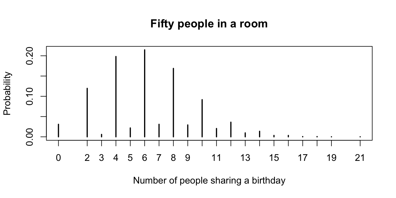
Figure 5.1: Probability mass function for the number of people who share a birthday with another person in a room with 50 people.

Looking at the pmf (in Figure 5.1), the most likely outcome is that 6 people in the room share a birthday with someone else, followed closely by 4, and then 8. Note that it is impossible for exactly one person to share a birthday with someone else in the room!

Example 5.8

You toss a coin 100 times. After each toss, either there have been more heads, more tails, or the same number of heads and tails. Let \(X\) be the number of times in the 100 tosses that there were more heads than tails. Estimate the pmf of \(X\).

Tryit 5.2

Before looking at the solution, guess whether the pmf of \(X\) will be centered around 50, or not.

We start by doing a single run of the experiment. The function cumsum accepts a numeric vector and returns the cumulative sum of the vector. So, cumsum(c(1, 3, -1)) would return c(1, 4, 3).

# flip 100 coins
coin_flips <- sample(c("H", "T"), 100, replace = TRUE)
coin_flips[1:10]

##  [1] "H" "H" "T" "T" "T" "T" "H" "H" "H" "T"

# calculate the cumulative number of heads or tails so far
num_heads <- cumsum(coin_flips == "H")
num_tails <- cumsum(coin_flips == "T")
num_heads[1:10]

##  [1] 1 2 2 2 2 2 3 4 5 5

num_tails[1:10]

##  [1] 0 0 1 2 3 4 4 4 4 5

# calculate the number of times there were more heads than tails
sum(num_heads > num_tails)

## [1] 53

Now, we put that inside of replicate.

X <- replicate(100000, {
  coin_flips <- sample(c("H", "T"), 100, replace = TRUE)
  num_heads <- cumsum(coin_flips == "H")
  num_tails <- cumsum(coin_flips == "T")
  sum(num_heads > num_tails)
})
pmf <- proportions(table(X))

When we have this many possible outcomes, it is easier to view a plot of the pmf than to look directly at the table of probabilities.

plot(pmf, ylab = "Probability", xlab = "More heads than tails")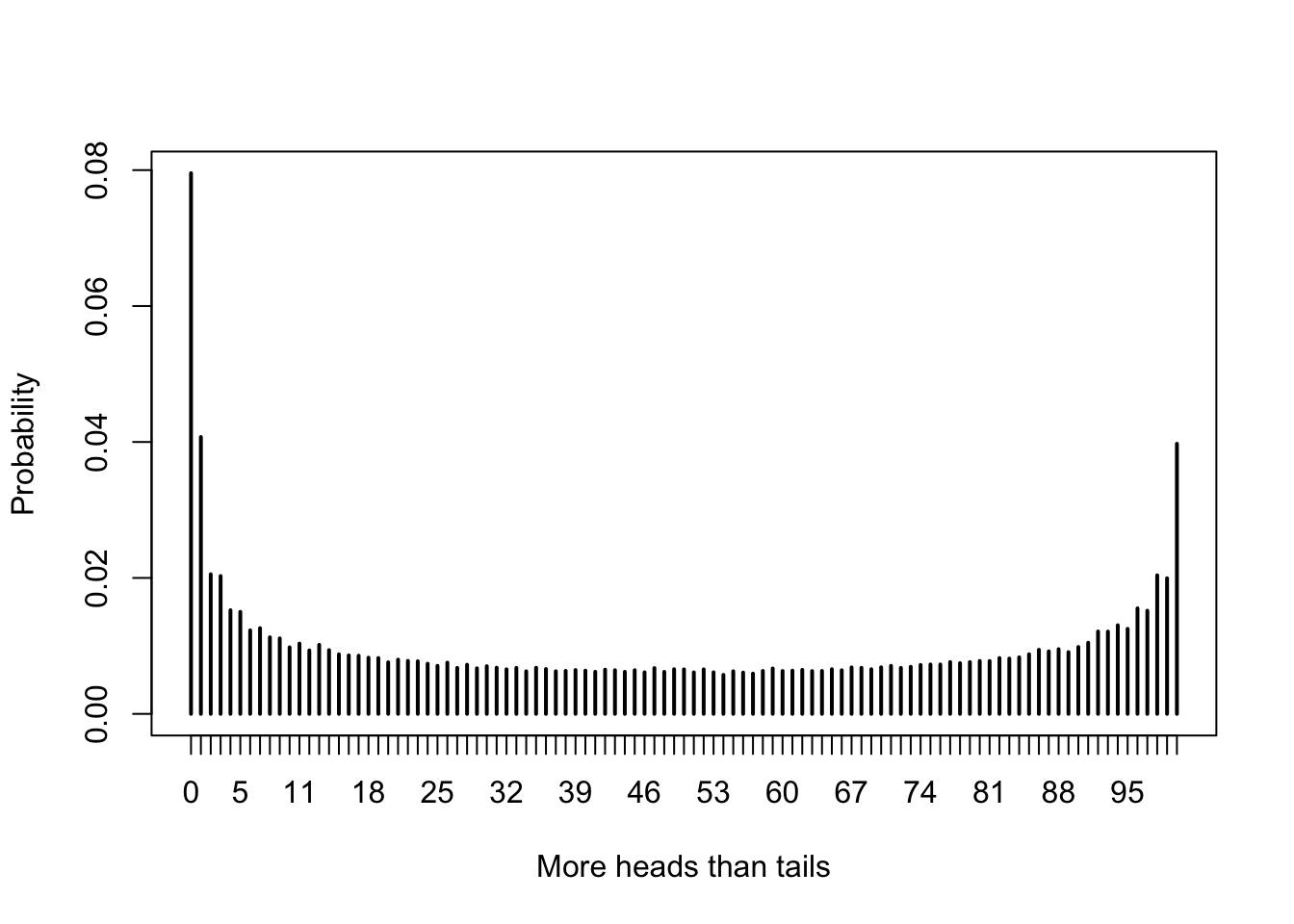

The most likely outcome (by far) is that there are never more heads than tails in the 100 tosses of the coin. This result can be surprising, even to experienced mathematicians.

Example 5.9

Suppose you have a bag full of marbles; 50 are red and 50 are blue. You are standing on a number line, and you draw a marble out of the bag. If you get red, you go left one unit. If you get blue, you go right one unit. This is called a random walk. You draw marbles up to 100 times, each time moving left or right one unit. Let \(X\) be the number of marbles drawn from the bag until you return to 0 for the first time. The rv \(X\) is called the first return time since it is the number of steps it takes to return to your starting position.

Estimate the pmf of \(X\).

First, simulate the steps of the walk, with 1 and -1 representing steps right and left.

movements <- sample(rep(c(1, -1), times = 50), 100, replace = FALSE)
movements[1:10]

##  [1]  1  1 -1 -1 -1 -1  1  1  1 -1

Next, use cumsum to calculate the cumulative sum of the steps. This vector gives the position of the walk at each step.

cumsum(movements)[1:10]

##  [1]  1  2  1  0 -1 -2 -1  0  1  0

The values where the cumulative sum is zero represent a return to the origin. Using which, we learn which steps of the walk were zero, and then find the first of these with min.

which(cumsum(movements) == 0)

## [1]   4   8  10  12  56  78  82  94 100

min(which(cumsum(movements) == 0))

## [1] 4

This results in a single value of the rv \(X\), in this case 4. To finish, we replicate the code and table it to compute the pmf.

X <- replicate(10000, {
  movements <- sample(rep(c(1, -1), times = 50), 100, replace = FALSE)
  min(which(cumsum(movements) == 0))
})
pmf <- proportions(table(X))
plot(pmf,
  main = "First return time for a 100 step random walk",
  xlab = "Steps to return",
  ylab = "Probability"
)

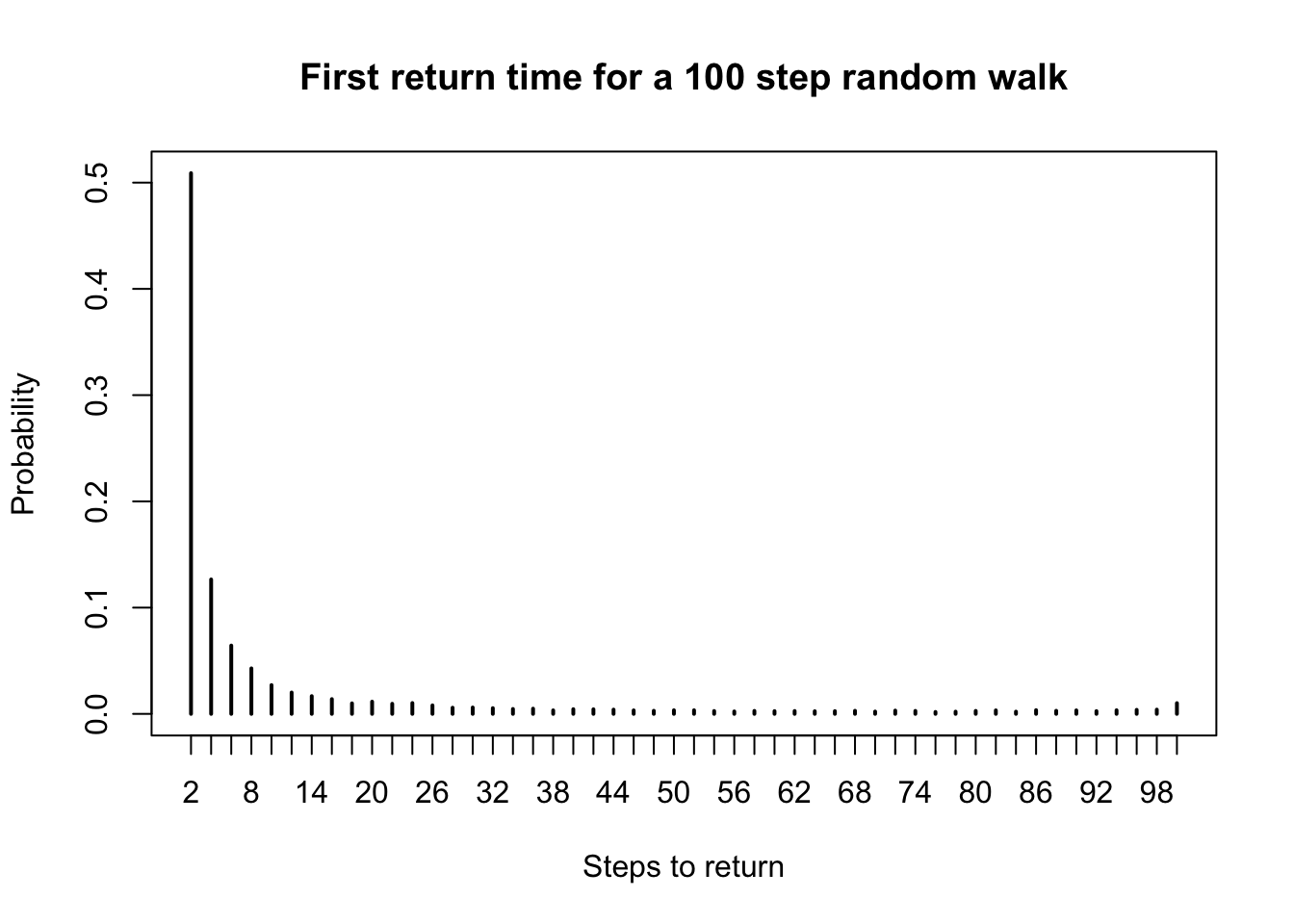
Only even return times are possible (why?). Half the time the first return is after two draws, one of each color. There is a slight bump near 100, when the bag of marbles empties out and the number of red and blue marbles drawn are forced to equalize.

5.3 Estimating continuous distributions

In this section, we show how to estimate the pdf of a continuous rv \(X\) via simulation. For discrete rvs, we used table to produce a count of each value that occurred in our simulation. These counts approximated the pmf. However, continuous rvs essentially never take the same value twice, so table is not helpful.

Instead, we divide the range of \(X\) into segments and count the number of values in each segment that appear in the simulation. These counts can be visualized by drawing a vertical bar over each segment of the range, with height corresponding to the count or proportion of values that appeared in that segment. The resulting graph is called a histogram and is easily produced with the R command hist.

For distributions where the pdf is continuous, we may also use density estimation. The height of the density estimation is a weighted sum of the distances to all of the data points in the sample. Places which are close to many data points will have higher density estimates, while places that are far from most data points will have lower density estimates. The R command for density estimation is density, and in this book we will only use the result of density estimation to produce a plot. The plot results in a smooth curve whose height approximates the pdf of the random variable.

Example 5.10

Estimate the pdf of \(2Z\) when \(Z\) is a standard normal random variable.

We simulate 10,000 values of a standard normal rv \(Z\) and then multiply by 2 to get 10,000 values sampled from \(2Z\).

Z <- rnorm(10000)
twoZ <- 2 * Z

We then use density to estimate and plot the pdf of the data:

plot(density(twoZ),
  main = "Density of 2Z",
  xlab = "2Z"
)

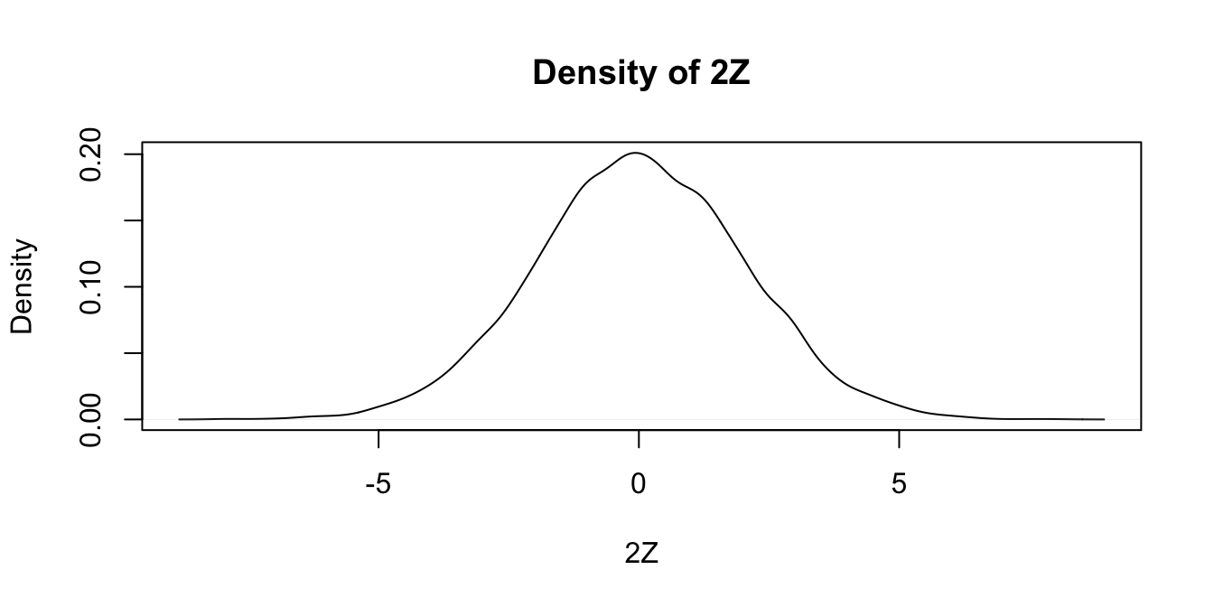
Notice that the most likely outcome of \(2Z\) seems to be 0, just as it is for \(Z\), but that the spread of the distribution of \(2Z\) is twice as wide as the spread of \(Z\).

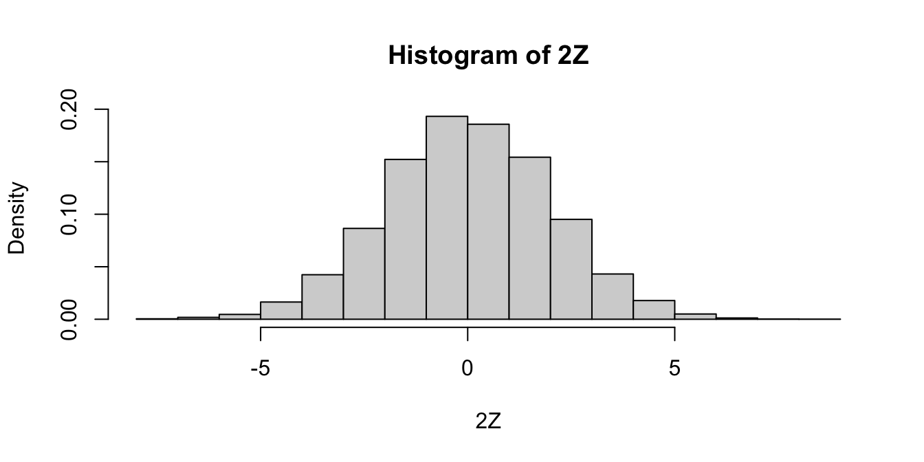
Alternatively, we could create a histogram of the data, using hist. We set probability = TRUE to adjust the scale on the \(y\)-axis so that the area of each rectangle in the histogram is the probability that the random variable falls in the interval given by the base of the rectangle.

hist(twoZ,
  probability = TRUE,
  main = "Histogram of 2Z",
  xlab = "2Z"
)

Given experimental information about a probability density, we wish to compare it to a known theoretical pdf. A direct way to make this comparison is to plot the estimated pdf on the same graph as the theoretical pdf. To add a curve to a histogram, density plot, or any plot, use the R function curve.

Example 5.11

Compare the pdf of \(2Z\), where \(Z\sim \text{Norm}(0,1)\) to the pdf of a normal random variable with mean 0 and standard deviation 2.

We already saw how to estimate the pdf of \(2Z\), we just need to plot the pdf of \(\text{Norm}(0,2)\) on the same graph. We show how to do this using both the histogram and the density plot approach. The pdf \(f(x)\) of \(\text{Norm}(0,2)\) is given in R by the function \(f(x) = \text{dnorm}(x,0,2)\).

hist(twoZ,
  probability = TRUE,
  main = "Density and histogram of 2Z",
  xlab = "2Z"
)
curve(dnorm(x, 0, 2), add = TRUE, col = "red")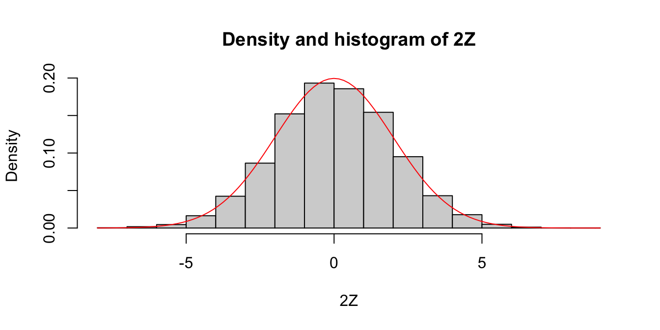

Since the area of each rectangle in the histogram is approximately the same as the area under the curve over the same interval, this is evidence that \(2Z\) is normal with mean 0 and standard deviation 2. Next, let’s look at the density estimation together with the true pdf of a normal rv with mean 0 and \(\sigma = 2\).

plot(density(twoZ),
  xlab = "2Z",
  main = "Density 2Z and Norm(0, 2)"
)
curve(dnorm(x, 0, 2), add = TRUE, col = "red")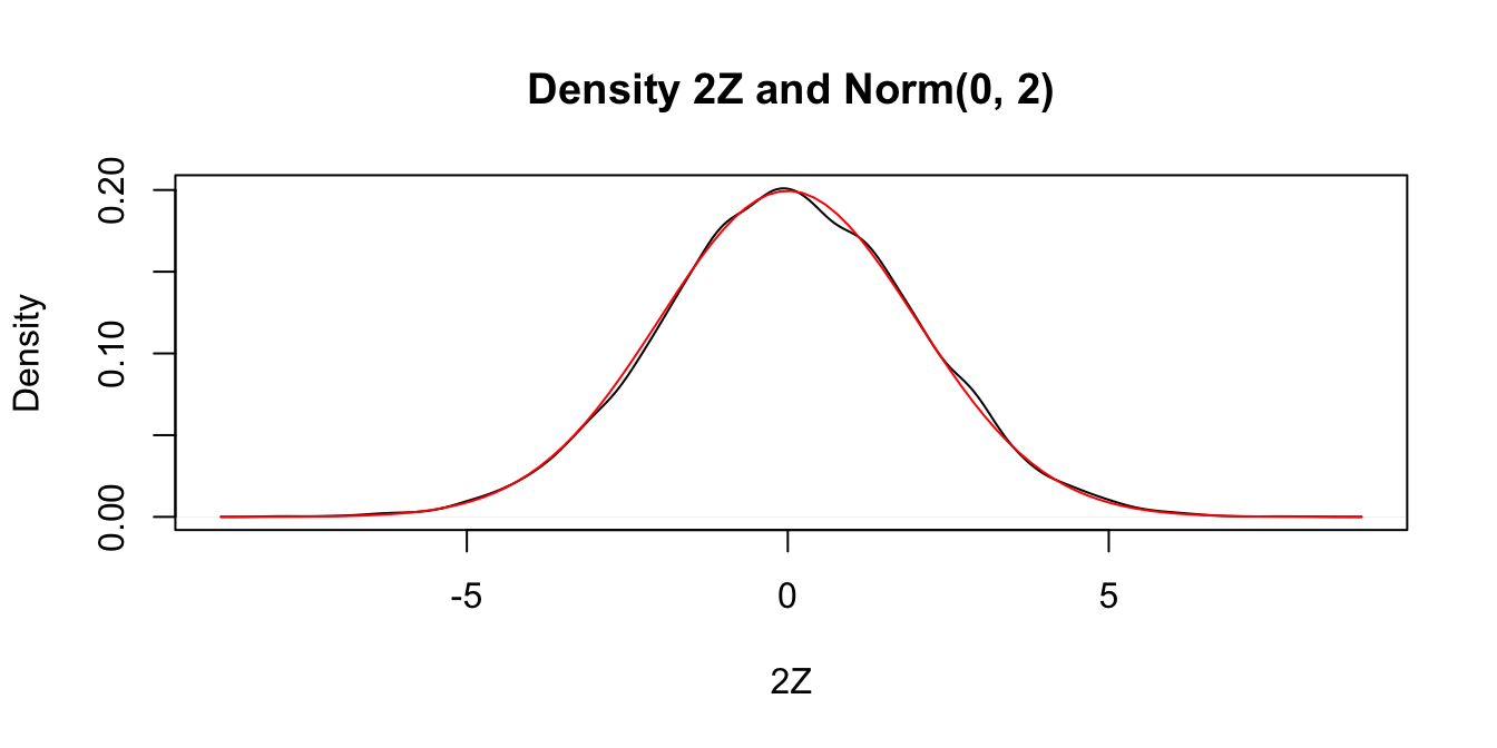

Wow! Those look really close to the same thing! This is again evidence that \(2Z \sim \text{Norm}(0, 2)\).

It would be a good idea to label the two curves in our plots, but that sort of finesse is easier with ggplot, which will be discussed in Chapter 7. Also in Chapter 7, we introduce qq plots, which are a more accurate (but less intuitive) way to compare continuous distributions.

Example 5.12

Estimate via simulation the pdf of \(W = \log\bigl(\left|Z\right|\bigr)\) when \(Z\) is standard normal.

W <- log(abs(rnorm(10000)))
plot(density(W),
  main = "Density of log|Z|",
  xlab = "log|Z|"
)

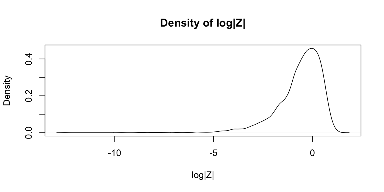
The simulations in Examples 5.10 and 5.12 worked well because the pdfs of \(2Z\) and of \(\log\bigl(\left|Z\right|\bigr)\) are continuous functions. For pdfs with discontinuities, density estimation of this type will misleadingly smooth out the jumps in the function.

Example 5.13

Estimate the pdf of \(X\) when \(X\) is uniform on the interval \([-1,1]\).

X <- runif(10000, -1, 1)
plot(density(X),
  main = "Density of Unif[-1,1]",
  xlab = "X"
)
curve(dunif(x, -1, 1), add = TRUE, col = "red")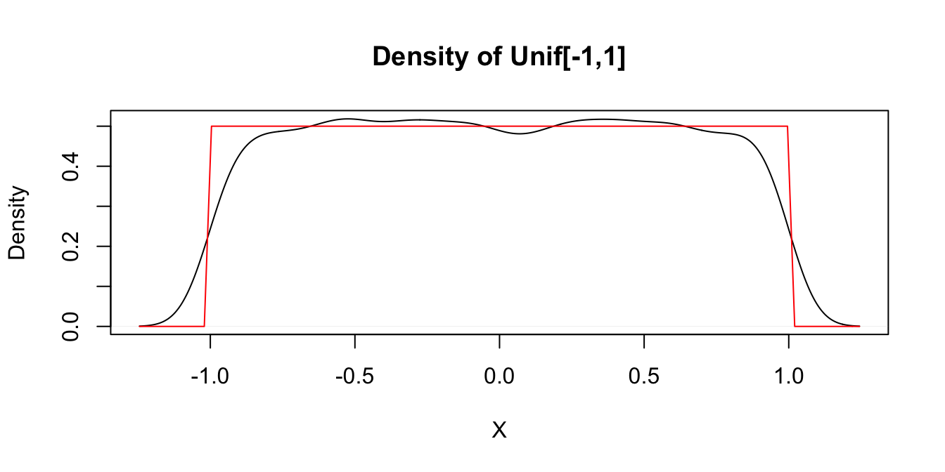

This distribution should be exactly 0.5 between -1 and 1, and zero everywhere else, as shown by the theoretical distribution in red. The simulation is reasonable in the middle, but the discontinuities at the endpoints are not shown well. Increasing the number of data points helps, but it does not fix the problem.

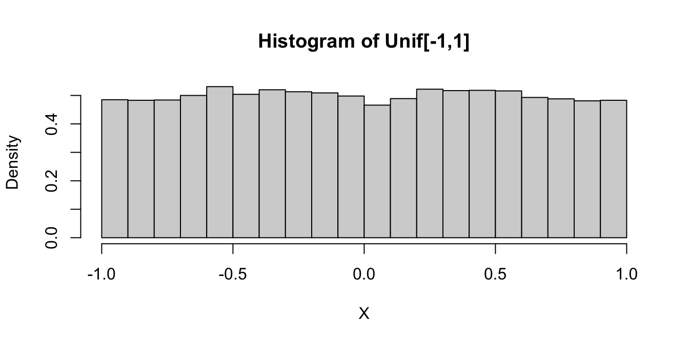
For this distribution, which has a jump discontinuity, using a histogram works better.

hist(X,
  probability = TRUE,
  main = "Histogram of Unif[-1,1]",
  xlab = "X"
)

We now use density estimation to give evidence of an important fact: the sum of normal random variables is still normal.

Example 5.14

Estimate the pdf of \(Z_1 + Z_2\) where \(Z_1\) and \(Z_2\) are independent standard normal random variables.

Z1 <- rnorm(10000)
Z2 <- rnorm(10000)
plot(density(Z1 + Z2),
  main = "Sum of two standard normal rvs",
  xlab = expression(Z[1] + Z[2])
)
curve(dnorm(x, 0, sqrt(2)), add = TRUE, col = "red")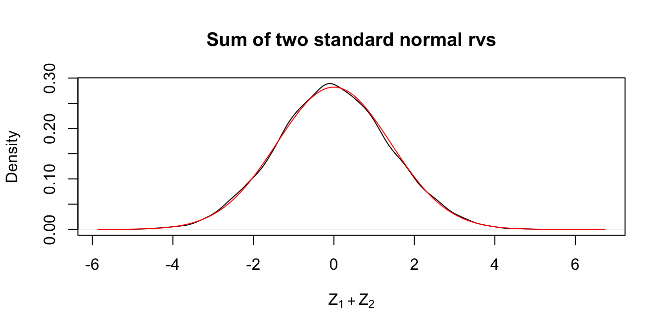

In the plot, the pdf for a \(\text{Norm}(0,\sqrt{2})\) rv is included. It appears that the sum of two standard normal random variables is again a normal random variable. The standard deviation is \(\sqrt{2}\) since \(\text{Var}(Z_1 + Z_2) = \text{Var}(Z_1) + \text{Var}(Z_2) = 2\) by Theorem 3.10.

Tryit 5.3

For \(Z_1\),\(Z_2\) independent standard normal, estimate the pdf of \(Z_1 - Z_2\) and see that it is also \(\text{Norm}(0,\sqrt{2})\).

Exercise 5.16 asks you to investigate the sum of two normal rvs which are not standard mean 0, sd 1, and see that their sum is normal as well. We will not prove that this is always true, but state it as the following:

Theorem 5.1

If \(X \sim \text{Norm}(\mu_X,\sigma_X)\) and \(Y \sim \text{Norm}(\mu_Y,\sigma_Y)\) are independent, then \(X+Y\) is normal with mean \(\mu_X + \mu_Y\) and variance \(\sigma_X^2 + \sigma_Y^2\).

More generally,

Theorem 5.2

Let \(X_1, \ldots, X_n\) be mutually independent normal random variables with means \(\mu_1, \ldots, \mu_n\) and standard deviations \(\sigma_1, \ldots, \sigma_n\). The random variable \[ \sum_{i = 1}^n a_i X_i \] is a normal random variable with mean \(\sum_{i = 1}^n a_i \mu_i\) and standard deviation \(\sqrt{\sum_{i = 1}^n a_i^2 \sigma_i^2}\).

Let’s meet an important distribution, the \(\chi^2\) (chi-squared) distribution. In fact, \(\chi^2\) is a family of distributions controlled by a parameter called the degrees of freedom, usually abbreviated df. The root name for a \(\chi^2\) rv is chisq, and dchisq requires the degrees of freedom to be specified using the df parameter.

Example 5.15

Let \(Z\) be a standard normal rv. Find the pdf of \(Z^2\) and compare it to the pdf of a \(\chi^2\) rv with one df on the same plot.

Z <- rnorm(10000)
hist(Z^2,
  probability = T,
  xlab = expression(Z^2)
)
curve(dchisq(x, df = 1), add = TRUE, col = "red")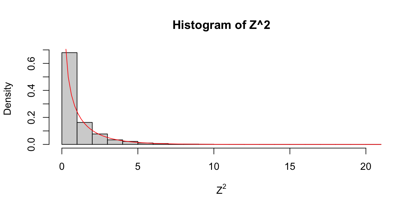

Figure 5.2: Estimated pdf of \(Z^2\) with the exact pdf of a \(\chi^2\) with 1 df overlaid in red.

As you can see in Figure 5.2, the estimated density follows the true histogram quite well. This is evidence that \(Z^2\) is, in fact, chi-squared. Notice that \(\chi^2\) with one df has a vertical asymptote at \(x = 0\).

Example 5.16

The sum of exponential random variables follows what is called a gamma distribution. The gamma distribution is represented in R via the root name gamma together with the typical prefixes dpqr. A gamma random variable has two parameters, the shape and the rate. It turns out (see Exercise 5.27) that:

1. The sum of independent gamma random variables with shapes \(\alpha_1\) and \(\alpha_2\) and the same rate \(\beta\) is again a gamma random variable with shape \(\alpha_1 + \alpha_2\) and rate \(\beta\).
2. A gamma random variable with shape 1 is an exponential random variable.

We check this in a simple case when \(X\) and \(Y\) are independent exponential random variables with rate 2. The sum \(W=X+Y\) should have a gamma distribution with shape 2 and rate 2.

We estimate the pdf of \(W = X + Y\), plot it, and overlay the pdf of a gamma random variable in Figure 5.3.

W <- replicate(10000, {
  X <- rexp(1, 2)
  Y <- rexp(1, 2)
  X + Y
})
hist(W,
  probability = TRUE,
  main = "Sum of exponentials is gamma",
  xlab = "X + Y",
  ylim = c(0, .72) # so the top of the curve is not clipped
)
curve(dgamma(x, shape = 2, rate = 2), add = TRUE, col = "red")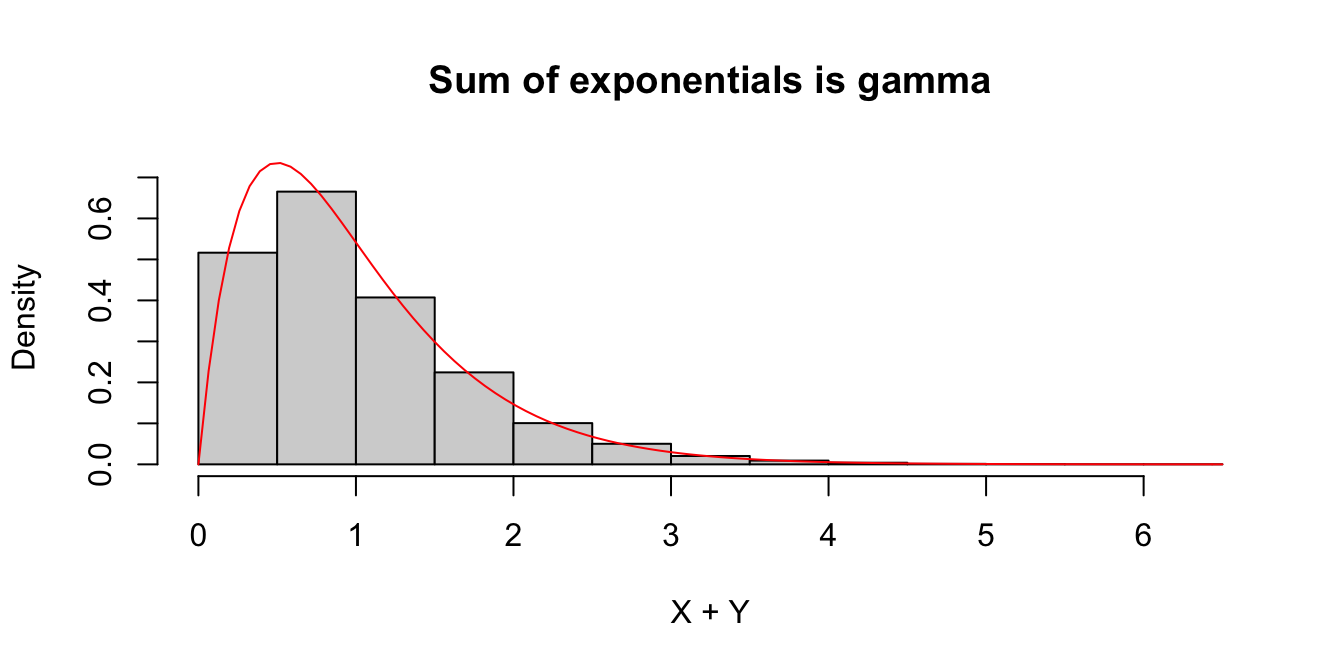

Figure 5.3: Histogram of the sum of two exponential variables \(X\) and \(Y\) with rate 2. The pdf for a gamma random variable with shape 2 and rate 2 is overlaid in red.

Example 5.17

Estimate the density of \(X_1 + X_2 + \cdots + X_{20}\) when all of the \(X_i\) are independent exponential random variables with rate 2.

This one is trickier and is our first example where it is easier to use replicate to create the data. Let’s build up the experiment that we are replicating from the ground up.

Here’s the experiment of summing 20 exponential rvs with rate 2:

sum(rexp(20, 2))

## [1] 8.325553

Now replicate it (10 times to test):

replicate(10, sum(rexp(20, 2)))

##  [1] 11.898357  6.407845  8.360866  9.297432 12.212909 11.200338
##  [7]  8.746138 10.663090 11.940880  8.289535

Of course, we don’t want to just replicate it 10 times; we need about 10,000 data points to get a good density estimate.

sumExpData <- replicate(10000, sum(rexp(20, 2)))
plot(density(sumExpData),
  main = "Density of sum of 20 exponentials",
  xlab = "X1 + ... + X20"
)
curve(dgamma(x, shape = 20, rate = 2), add = TRUE, col = "red")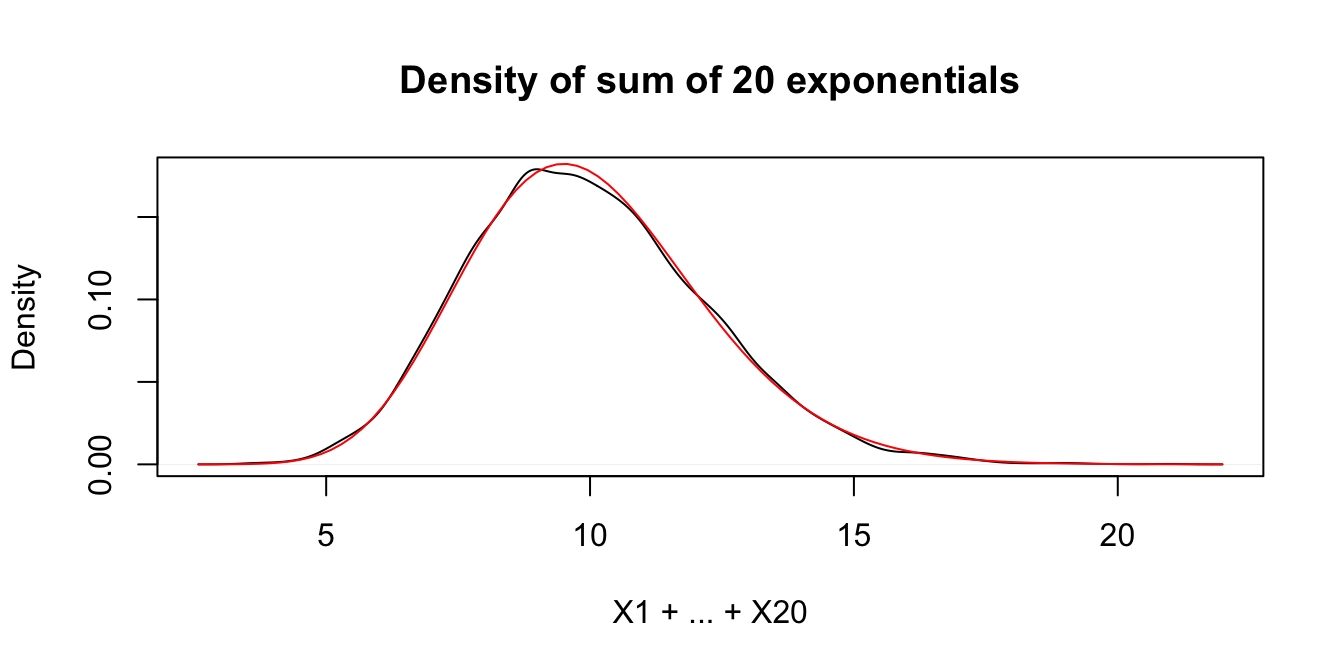

As explained in Example 5.16, this is exactly a gamma random variable with rate 2 and shape 20, and it is also starting to look like a normal random variable! Exercise 5.17 asks you to fit a normal curve to this distribution.

5.4 Central Limit Theorem

Definition 5.18

Random variables \(X_1,\ldots,X_n\) are called independent and identically distributed or iid if the variables are mutually independent, and each \(X_i\) has the same probability distribution.

All of R’s random generation functions (rnorm, rexp, etc.) produce samples from iid random variables. In the real world, iid rvs are produced by taking a random sample of size \(n\) from a population. Ideally, this sample would be obtained by numbering all members of the population and then using a random number generator to select members for the sample. As long as the population size is much larger than \(n\), the sampled values will be independent, and all will have the same probability distribution as the population distribution. However, in practice it is quite difficult to produce a true random sample from a real population, and failure to sample randomly can introduce error into mathematical results that depend on the assumption that random variables are iid.

Definition 5.19

Let \(X_1, \dotsc, X_n\) be a random sample. A random variable \(Y = h(X_1, \dotsc, X_n)\) that is derived from the random sample is called a sample statistic or sometimes just a statistic. The probability distribution of \(Y\) is called a sampling distribution.

Three of the most important statistics are the sample mean, sample variance, and sample standard deviation.

Definition 5.20

Assume \(X_1,\ldots,X_n\) are independent and identically distributed. Define:

• The sample mean \[ \overline{X} = \frac{X_1 + \dotsb + X_n}{n}. \]
• The sample variance \[ S^2 = \frac 1{n-1} \sum_{i=1}^n (X_i - \overline{X})^2 \]
• The sample standard deviation is \(S\), the square root of the sample variance.

These three statistics are computed in R with the commands mean, var, and sd that we have been using all along.

A primary goal of statistics is to learn something about a population (the distribution of the \(X_i\)’s) by studying sample statistics. We can make precise statements about a population from a random sample because it is possible to describe the sampling distributions of statistics like \(\overline{X}\) and \(S\) even in the absence of information about the distribution of the \(X_i\). The most important example of this phenomenon is the Central Limit Theorem, which is fundamental to statistical reasoning.

We first establish basic properties of the distribution of the sample mean.

Proposition 5.1

If \(X_1,\ldots,X_n\) are iid with mean \(\mu\) and standard deviation \(\sigma\), then the sample mean \(\overline{X}\) has mean and variance given by \[ E[\overline{X}] = \mu \] \[ \text{Var}(\overline{X}) = \sigma^2/n \]

Proof:

From linearity of expected value (Theorem 3.8), \[ E[\overline{X}] = E\left [\frac{X_1 + \dotsb X_n}{n}\right ] = \frac{1}{n}\Bigl(E[X_1] + \dotsb + E[X_n]\Bigr) = \frac{1}{n}(n\mu) = \mu. \]

Since the \(X_i\) are mutually independent, Theorem 3.10 applies and: \[ \text{Var}[\overline{X}] = \text{Var}\left(\frac{1}{n} \sum_i X_i\right) = \frac{1}{n^2}\text{Var}\left(\sum_i X_i\right) = \frac{1}{n^2}\sum_i \text{Var}(X_i) = \frac{1}{n^2}\cdot n \sigma^2 = \frac{\sigma^2}{n}\]

From Proposition 5.1, the random variable \(\frac{\overline{X} - \mu}{\sigma/\sqrt{n}}\) has mean 0 and standard deviation 1. When the population is normally distributed, Theorem 5.1 implies the following:

Proposition 5.2

If \(X_1, \dotsc, X_n\) are iid normal, then \(\frac{\overline{X} - \mu}{\sigma/\sqrt{n}} = Z\), where \(Z\) is a standard normal rv.

Remarkably, for large sample sizes we can still describe the distribution of \(\frac{\overline{X} - \mu}{\sigma/\sqrt{n}}\) even when we don’t know that the population is normal. This is the Central Limit Theorem.

Theorem 5.3 (Central Limit Theorem)

Let \(X_1,\ldots,X_n\) be iid rvs with finite mean \(\mu\) and standard deviation \(\sigma\). Then \[ \frac{\overline{X} - \mu}{\sigma/\sqrt{n}} \to Z \qquad \text{as}\ n \to \infty \] where \(Z\) is a standard normal rv.

We will not prove Theorem 5.3, but we will do simulations for several examples. They will all follow a similar format.

Example 5.21

Let \(X_1,\ldots,X_{30}\) be independent Poisson random variables with rate 2. From our knowledge of the Poisson distribution, each \(X_i\) has mean \(\mu = 2\) and standard deviation \(\sigma = \sqrt{2}\). Assuming \(n = 30\) is a large enough sample size, the Central Limit Theorem says that \[ Z = \frac{\overline{X} - 2}{\sqrt{2}/\sqrt{30}} \] will be approximately normal with mean 0 and standard deviation 1. Let us check this with a simulation.

This is a little bit more complicated than our previous examples, but the idea is still the same. We create an experiment which computes \(\overline{X}\) and then transforms it by subtracting 2 and dividing by \(\sqrt{2}/\sqrt{30}\).

Here is a single experiment:

Xbar <- mean(rpois(30, 2))
(Xbar - 2) / (sqrt(2) / sqrt(30))

## [1] 0.1290994

Now, we replicate and plot:

Z <- replicate(10000, {
  Xbar <- mean(rpois(30, 2))
  (Xbar - 2) / (sqrt(2) / sqrt(30))
})

plot(density(Z),
  main = "Standardized sum of 30 Poisson rvs", xlab = "Z"
)
curve(dnorm(x), add = TRUE, col = "red")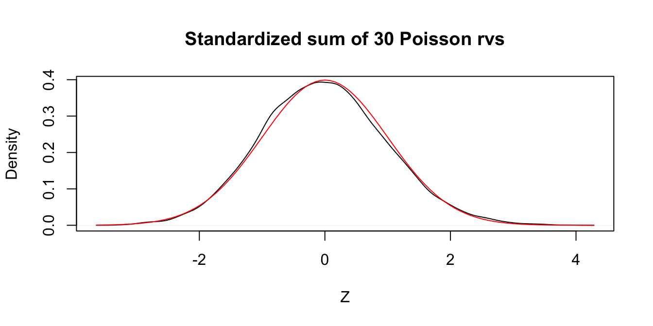

Figure 5.4: Standardized sum of 30 Poisson random variables compared to a standard normal rv.

In Figure 5.4 we see very close agreement between the simulated density of \(Z\) and the standard normal density curve.

Example 5.22

Let \(X_1,\ldots,X_{50}\) be independent exponential random variables with rate 1/3. From our knowledge of the exponential distribution, each \(X_i\) has mean \(\mu = 3\) and standard deviation \(\sigma = 3\). The Central Limit Theorem says that \[ Z = \frac{\overline{X} - 3}{3/\sqrt{n}} \] is approximately normal with mean 0 and standard deviation 1 when \(n\) is large. We check this with a simulation in the case \(n = 50\). The resulting plot, in Figure 5.5, shows that even with \(n=50\) a sum of exponential random variables is still slightly skew to the right.

Z <- replicate(10000, {
  Xbar <- mean(rexp(50, 1 / 3))
  (Xbar - 3) / (3 / sqrt(50))
})

plot(density(Z),
  main = "Standardized sum of 50 exponential rvs", xlab = "Z"
)
curve(dnorm(x), add = TRUE, col = "red")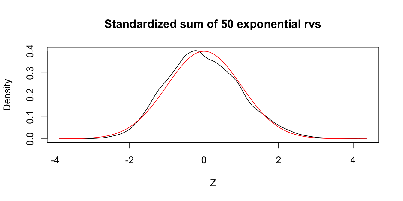

Figure 5.5: Standardized sum of 50 exponential random variables compared to a standard normal rv.

The Central Limit Theorem says that, if you take the mean of a large number of independent samples, then the distribution of that mean will be approximately normal. How large does \(n\) need to be in practice?

• If the population you are sampling from is symmetric with no outliers, a good approximation to normality appears after as few as 15-20 samples.
• If the population is moderately skewed, such as exponential or \(\chi^2\), then it can take between 30-50 samples before getting a good approximation.
• Data with extreme skewness, such as some financial data where most entries are 0, a few are small, and even fewer are extremely large, may not be appropriate for the Central Limit Theorem even with 1000 samples (see Example 5.23).

There are versions of the Central Limit Theorem available when the \(X_i\) are not iid, but outliers of sufficient size will cause the distribution of \(\overline{X}\) to not be normal, see Exercise 5.34.

Example 5.23

A distribution for which sample size of \(n = 1000\) is not sufficient for good approximation via normal distributions.

We create a distribution that consists primarily of zeros, but has a few modest sized values and a few large values:

# Start with lots of zeros
skewdata <- replicate(2000, 0)
# Add a few moderately sized values
skewdata <- c(skewdata, rexp(200, 1 / 10))
# Add a few large values
skewdata <- c(skewdata, seq(100000, 500000, 50000))

mu <- mean(skewdata)
sig <- sd(skewdata)

We use sample to take a random sample of size \(n\) from this distribution. We take the mean, subtract the true mean of the distribution, and divide by \(\sigma/\sqrt{n}\). We replicate that 10,000 times to estimate the sampling distribution. Here is the code we use to generate the sample and produce the plots shown in Figure 5.6.

Z <- replicate(10000, {
  Xbar <- mean(sample(skewdata, 100, TRUE))
  (Xbar - mu) / (sig / sqrt(100))
})
hist(Z,
  probability = TRUE,
  main = "100 Samples",
  xlab = "Z"
)
curve(dnorm(x), add = TRUE, col = "red")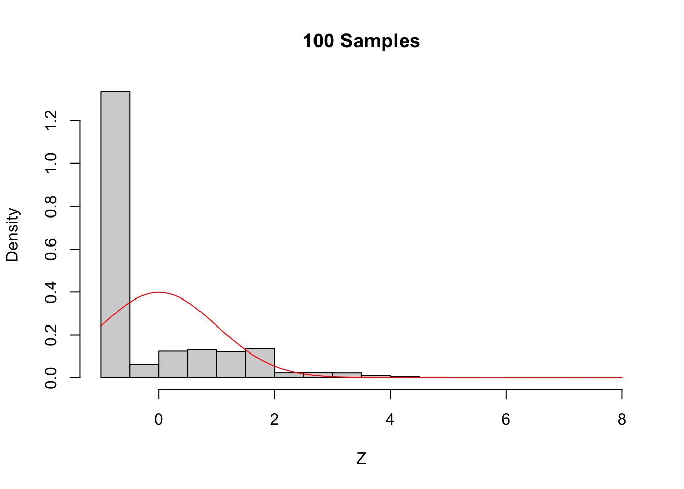

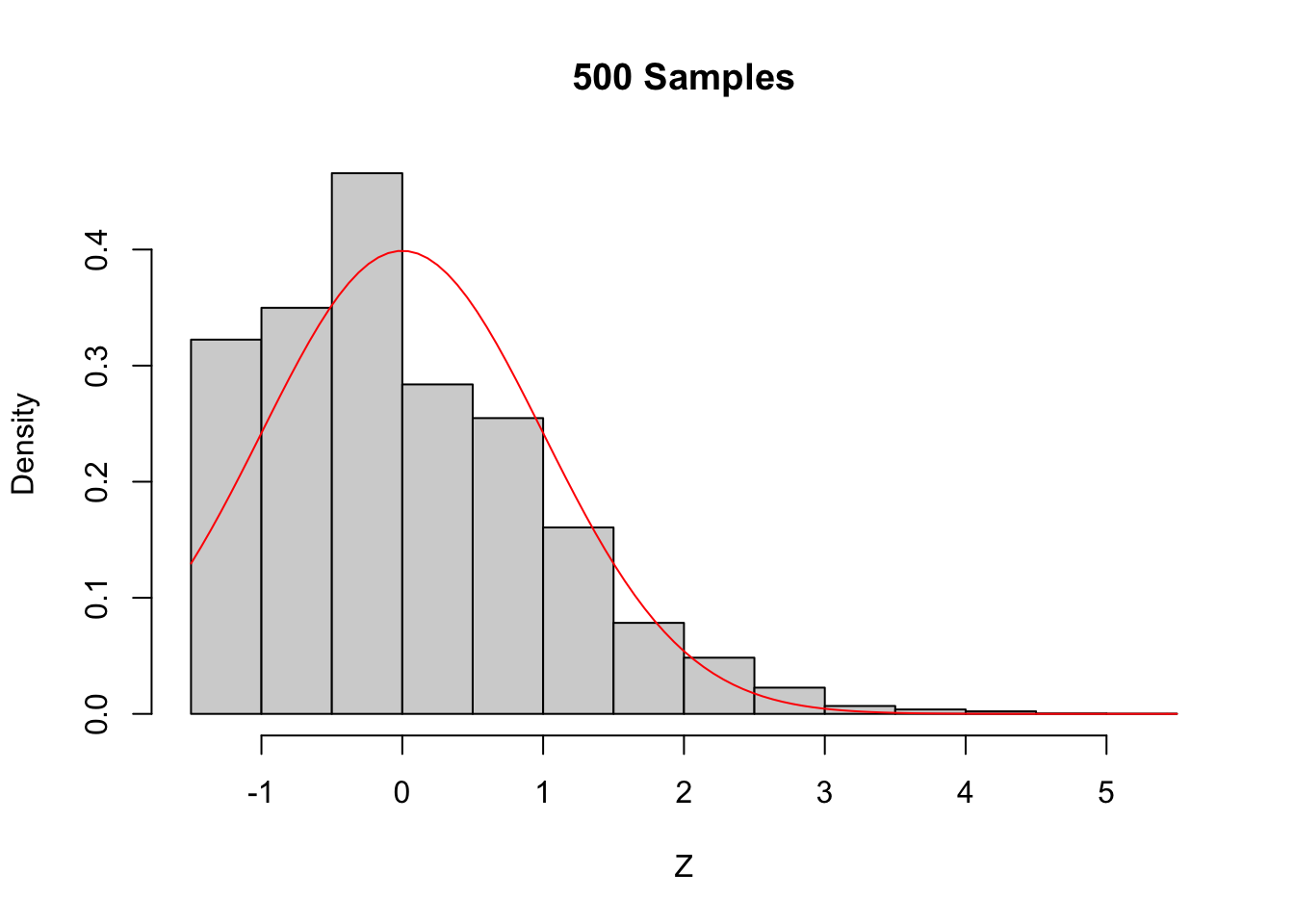
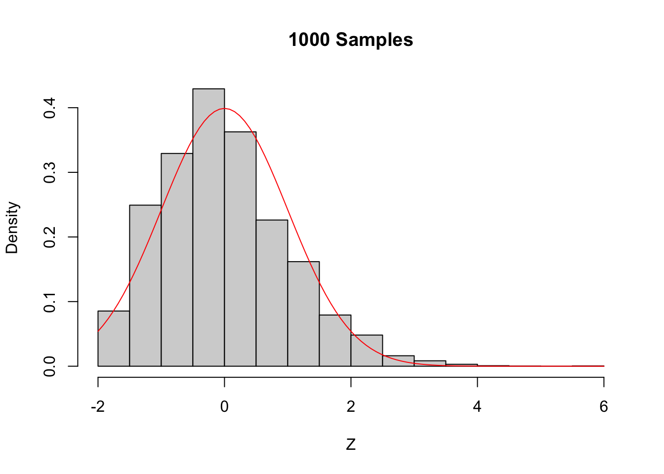
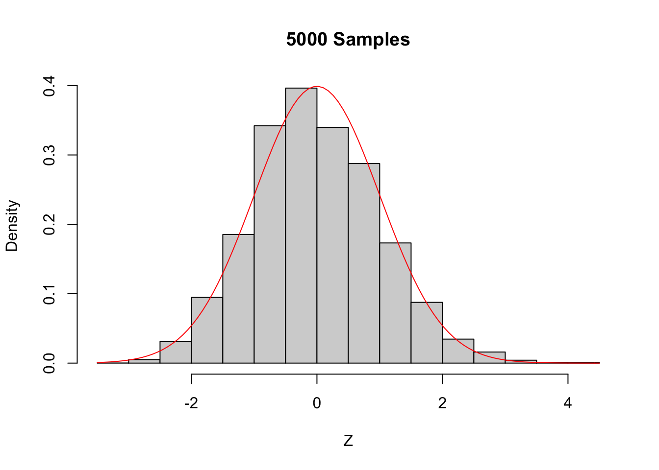
Figure 5.6: The Central Limit Theorem in action for an extremely skew population.

Even with a sample size of 1000, the density still fails to be normal, especially the lack of left tail. Of course, the Central Limit Theorem is still true, so \(\overline{X}\) must become approximately normal if we choose \(n\) large enough. When \(n=5000\) there is still a slight skewness in the distribution, but it is finally close to normal.

5.5 Sampling distributions

We describe the \(\chi^2\), \(t\), and \(F\) distributions, which are examples of distributions that are derived from random samples from a normal distribution. The emphasis is on understanding the relationships between the random variables and how they can be used to describe distributions related to the sample statistics \(\overline{X}\) and \(S\). Your goal should be to get comfortable with the idea that sample statistics have known distributions. You may not be able to prove relationships that you see later in this book, but with careful study of this chapter you won’t be surprised, either. We will use density estimation extensively to illustrate the relationships.

5.5.1 The \(\chi^2\) distribution

Definition 5.24

Let \(Z\) be a standard normal random variable. An rv with the same distribution as \(Z^2\) is called a Chi-squared random variable with one degree of freedom.

Let \(Z_1, \dotsc, Z_n\) be \(n\) iid standard normal random variables. An rv with the same distribution as \(Z_1^2 + \dotsb + Z_n^2\) is called a Chi-squared random variable with \(n\) degrees of freedom.

Remark

The sum of \(n\) independent \(\chi^2\) rvs with 1 degree of freedom is a \(\chi^2\) rv with \(n\) degrees of freedom. More generally, the sum of a \(\chi^2\) with \(\nu_1\) degrees of freedom and a \(\chi^2\) rv with \(\nu_2\) degrees of freedom is \(\chi^2\) rv with \(\nu_1 + \nu_2\) degrees of freedom.

Let’s check by estimating pdfs that the sum of a \(\chi^2\) rv with 2 df and a \(\chi^2\) rv with 3 df is a \(\chi^2\) rv with 5 df.

X <- rchisq(10000, 2)
Y <- rchisq(10000, 3)
hist(X + Y,
  probability = TRUE,
  main = "Sum of chi^2 random variables"
)
curve(dchisq(x, df = 5), add = TRUE, col = "red")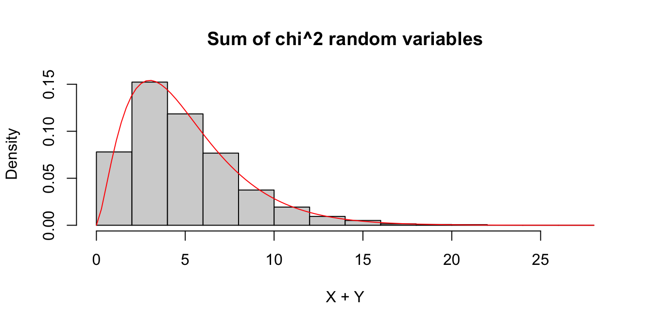

The \(\chi^2\) distribution is important for understanding the sample variance \(S^2\).

Theorem 5.4

If \(X_1,\ldots,X_n\) are iid normal rvs with mean \(\mu\) and standard deviation \(\sigma\), then \[ \frac{n-1}{\sigma^2} S^2 \] has a \(\chi^2\) distribution with \(n-1\) degrees of freedom.

We provide a heuristic and a simulation as evidence that Theorem 5.4 is true. Additionally, in Exercise 5.40 you are asked to prove Theorem 5.4 in the case that \(n = 2\).

Heuristic argument: Note that \[ \frac{n-1}{\sigma^2} S^2 = \frac 1{\sigma^2}\sum_{i=1}^n \left(X_i - \overline{X}\right)^2 \\ = \sum_{i=1}^n \left(\frac{X_i - \overline{X}}{\sigma}\right)^2 \] Now, if we had \(\mu\) in place of \(\overline{X}\) in the above equation, we would have exactly a \(\chi^2\) with \(n\) degrees of freedom. Replacing \(\mu\) by its estimate \(\overline{X}\) reduces the degrees of freedom by one, but it remains \(\chi^2\).

For the simulation, we estimate the density of \(\frac{n-1}{\sigma^2} S^2\) and compare it to that of a \(\chi^2\) with \(n-1\) degrees of freedom, in the case that \(n = 4\), \(\mu = 5\) and \(\sigma = 9\).

S2 <- replicate(10000, 3 / 81 * sd(rnorm(4, 5, 9))^2)
hist(S2,
  probability = TRUE,
  main = "Sample variance compared to chi^2",
  xlab = expression(S^2),
  ylim = c(0, .25)
)
curve(dchisq(x, df = 3), add = TRUE, col = "red")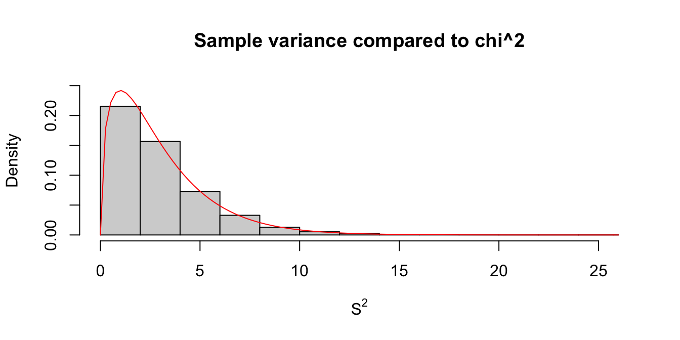

5.5.2 The \(t\) distribution

This section introduces Student’s \(t\) distribution. The distribution is named after William Gosset, who published under the pseudonym “Student” while working at the Guinness Brewery in the early 1900’s.

Definition 5.25

If \(Z\) is a standard normal random variable, \(\chi^2_\nu\) is a Chi-squared rv with \(\nu\) degrees of freedom, and \(Z\) and \(\chi^2_\nu\) are independent, then

\[ t_\nu = \frac{Z}{\sqrt{\chi^2_\nu/\nu}} \]

is distributed as a \(t\) random variable with \(\nu\) degrees of freedom.

The \(t\) distributions are symmetric around zero and bump-shaped, like the normal distribution, but the \(t\) distributions are heavy tailed. The heavy tails mean that \(t\) random variables have higher probability of being far from 0 than normal random variables do, in the sense that \[ \lim_{M \to \infty} \frac{P(|T| > M)}{P(|Z| > M)} = \infty \] for any normal rv \(Z\) and \(T\) having any \(t\) distribution.

The \(t\) distribution will play an important role in Chapter 8, where it appears as the result of random sampling. Theorem 5.5 establishes the connection between a random sample \(X_1,\dotsc,X_n\) and the \(t\) distribution.

Theorem 5.5

If \(X_1,\ldots,X_n\) are iid normal rvs with mean \(\mu\) and sd \(\sigma\), then \[ \frac{\overline{X} - \mu}{S/\sqrt{n}} \] is \(t\) with \(n-1\) degrees of freedom.

Proof:

\[ \frac{Z}{\sqrt{\chi^2_{n-1}/n}} = \frac{\overline{X} - \mu}{\sigma/\sqrt{n}}\cdot\sqrt{\frac{\sigma^2 (n-1)}{S^2(n-1)}}\\ = \frac{\overline{X} - \mu}{S/\sqrt{n}} \] Where we have used that \((n - 1) S^2/\sigma^2\) is \(\chi^2\) with \(n - 1\) degrees of freedom.

Since the mean and standard deviation of \(\overline{X}\) are \(\mu\) and \(\sigma/\sqrt{n}\), the random variable \(\frac{\overline{X} - \mu}{\sigma/\sqrt{n}}\) is \(\text{Norm}(0,1)\). Replacing the denominator \(\sigma/\sqrt{n}\) with the random variable \(S/\sqrt{n}\) changes the distribution from normal to \(t\).

Definition 5.26

The random variable \(S/\sqrt{n}\) is the standard error of \(\overline{X}\).

Example 5.27

Estimate the pdf of \(\frac{\overline{X} - \mu}{S/\sqrt{n}}\) in the case that \(X_1,\ldots,X_6\) are iid normal with mean 3 and standard deviation 4, and compare it to the pdf of the appropriate \(t\) random variable.

tData <- replicate(10000, {
  X <- rnorm(6, 3, 4)
  (mean(X) - 3) / (sd(X) / sqrt(6))
})
hist(tData,
  probability = TRUE,
  ylim = c(0, .37),
  main = "Histogram of t",
  xlab = "t"
)
curve(dt(x, df = 5), add = TRUE, col = "red")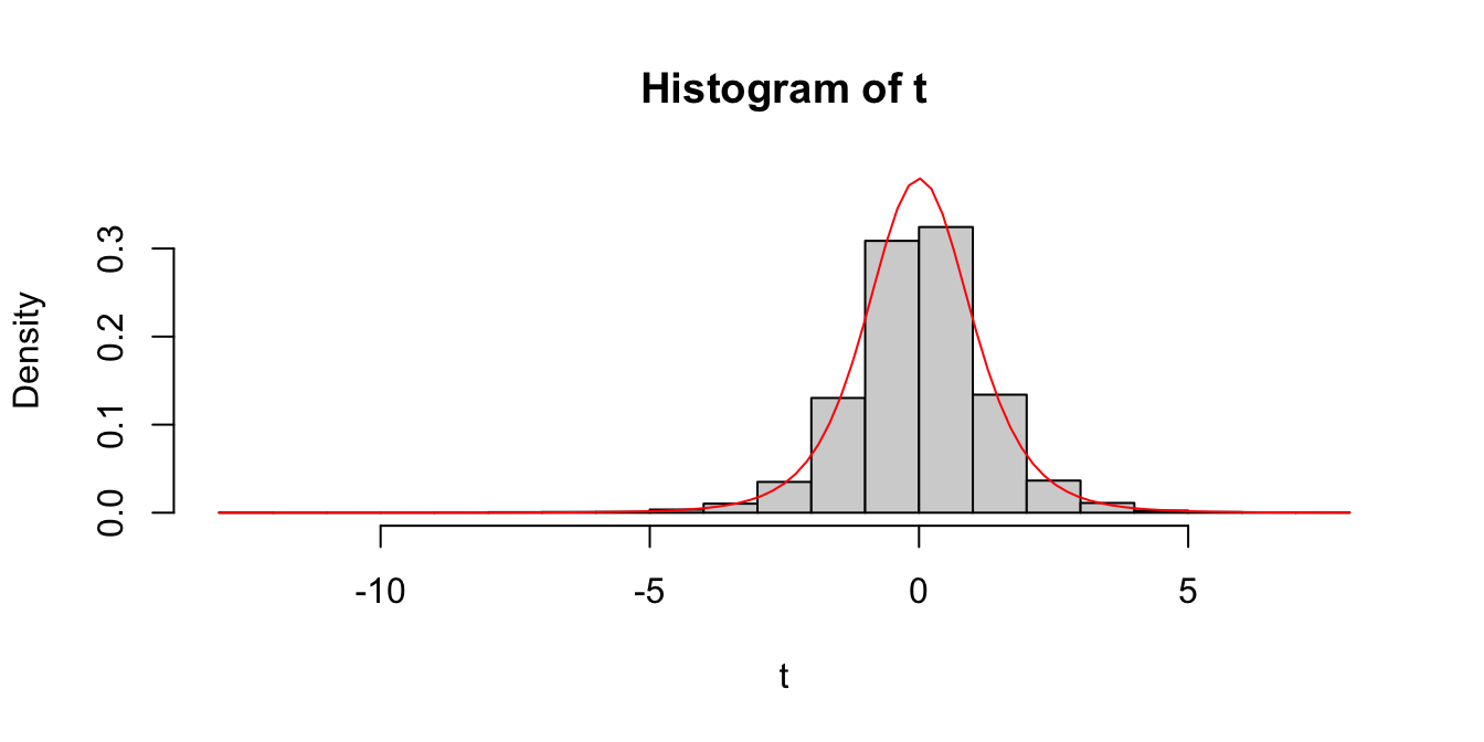

We see a very good agreement.

5.5.3 The \(F\) distribution

An \(F\) distribution has the same density function as \[ F_{\nu_1, \nu_2} = \frac{\chi^2_{\nu_1}/\nu_1}{\chi^2_{\nu_2}/\nu_2} \] when \(\chi^2_{\nu_1}\) and \(\chi^2_{\nu_2}\) are independent. We say \(F\) has \(\nu_1\) numerator degrees of freedom and \(\nu_2\) denominator degrees of freedom.

One example of this type is: \[ \frac{S_1^2/\sigma_1^2}{S_2^2/\sigma_2^2} \] where \(X_1,\ldots,X_{n_1}\) are iid normal with standard deviation \(\sigma_1\) and \(Y_1,\ldots,Y_{n_2}\) are iid normal with standard deviation \(\sigma_2.\)

5.5.4 Summary

This chapter has introduced the key variables associated with sampling distributions. Here, we summarize the relationships among these variables for ease of reference.

Suppose \(X\) is normal with mean \(\mu\) and sd \(\sigma\). Then:

• \(aX+ b\) is normal with mean \(a\mu + b\) and standard deviation \(a\sigma\).
• \(\displaystyle \frac{X - \mu}{\sigma}\sim Z\), where \(Z\) is standard normal.

Given a random sample \(X_1,\ldots,X_n\) with mean \(\mu\) and standard deviation \(\sigma\),

• \(\displaystyle \frac{\overline{X} - \mu}{\sigma/\sqrt{n}} \sim Z\) if the \(X_i\) are normal.
• \(\displaystyle \lim_{n\to \infty} \frac{\overline{X} - \mu}{\sigma/\sqrt{n}} \sim Z\) if the \(X_i\) have finite variance (the Central Limit Theorem).

To understand the sample mean \(\overline{X}\) and standard deviation \(S\), we introduced:

• \(\displaystyle \chi^2_\nu\) the chi-squared random variable with \(\nu\) degrees of freedom.
• \(\displaystyle t_\nu\) the \(t\) random variable with \(\nu\) degrees of freedom.
• \(\displaystyle F_{\nu, \mu}\) the \(F\) random variable with \(\nu\) and \(\mu\) degrees of freedom.

These satisfy:

• \(\displaystyle Z^2 \sim \chi^2_1\).
• \(\displaystyle \chi^2_\nu + \chi^2_\eta \sim \chi^2_{\nu + \eta}\) if independent.
• \(\displaystyle \frac{(n-1)S^2}{\sigma^2} \sim \chi^2_{n-1}\) when \(X_1,\ldots,X_n\) iid normal.
• \(\displaystyle \frac Z{\sqrt{\chi^2_\nu/\nu}} \sim t_\nu\) if independent.
• \(\displaystyle \frac{\overline{X} - \mu}{S/\sqrt{n}}\sim t_{n-1}\) when \(X_1,\ldots,X_n\) iid normal.
• \(\displaystyle \frac{\chi^2_\nu/\nu}{\chi^2_\mu/\mu} \sim F_{\nu, \mu}\) if independent.
• \(\displaystyle \frac{S_1^2/\sigma_1^2}{S_2^2/\sigma_2^2} \sim F_{n_1 - 1, n_2 - 1}\) if \(X_1,\ldots,X_{n_1}\) iid normal with sd \(\sigma_1\) and \(Y_1,\ldots,Y_{n_2}\) iid normal with sd \(\sigma_2\).

5.6 Point estimators

This section explores the definition of sample mean and (especially) sample variance, in the more general context of point estimators and their properties.

Suppose that a random variable \(X\) depends on some parameter \(\theta\). In many instances we do not know \(\theta,\) but are interested in estimating it from observations of \(X\).

Definition 5.28

If \(X_1, \ldots, X_n\) are iid with the same distribution as \(X\), then a point estimator for \(\theta\) is a function \(\hat\theta = \hat\theta(X_1, \ldots, X_n)\).

Typically the value of \(\hat \theta\) represents our best estimate of the parameter \(\theta\), based on the data. Note that \(\hat \theta\) is a random variable, and since \(\hat \theta\) is derived from \(X_1, \dotsc, X_n\), \(\hat\theta\) is a sample statistic and has a sampling distribution.

The two point estimators that we examine in this section are the sample mean and sample variance. The sample mean \(\overline{X}\) is a point estimator for the mean of a random variable, and the sample variance \(S^2\) is a point estimator for the variance of an rv.

Suppose we want to understand a random variable \(X\). We collect a random sample of data \(x_1,\ldots,x_n\) from the \(X\) distribution. We then imagine a new discrete random variable \(X_0\) which samples uniformly from these \(n\) data points.

The variable \(X_0\) satisfies \(P(X_0 = x_i) = 1/n\), and so its mean is \[ E[X_0] = \frac 1n \sum_{i=1}^n x_i = \overline{x}. \]

Since \(X_0\) incorporates everything we know about \(X\), it is reasonable to use the mean of \(X_0\) as a point estimator for \(\mu\), the mean of \(X\):

\[ \hat \mu = \overline{X} = \frac 1n \sum_{i=1}^n X_i \]

Continuing in the same way,

\[ \sigma^2 = E[(X_0 - \mu)^2] = \frac 1n \sum_{i=1}^n (x_i - \mu)^2 \]

This works just fine as long as \(\mu\) is known. However, most of the time, we do not know \(\mu\) and we must replace the true value of \(\mu\) with our estimate from the data. There is a heuristic “degrees of freedom” that each time you replace a parameter with an estimate of that parameter, you divide by one less. Following that heuristic, we obtain \[ \hat \sigma^2 = S^2 = \frac 1{n-1} \sum_{i=1}^n (x_i - \overline{x})^2 \]

5.6.1 Properties of point estimators

The point estimators \(\overline{X}\) for \(\mu\) and \(S^2\) for \(\sigma^2\) are random variables themselves, since they are computed using a random sample from a distribution. As such, they also have distributions, means and variances. One desirable property of point estimators is that they be unbiased.

Definition 5.29

A point estimator \(\hat \theta\) for \(\theta\) is an unbiased estimator if \(E[\hat \theta] = \theta\).

Intuitively, “unbiased” means that the estimator does not consistently underestimate or overestimate the parameter it is estimating. If we were to estimate the parameter over and over again, the average value of the estimates would converge to the correct value of the parameter.

Example 5.30

Let \(X_1,\ldots, X_{5}\) be a random sample from a normal distribution with mean 1 and variance 4. Compute \(\overline{X}\) based on the random sample.

mean(rnorm(5, 1, 2))

## [1] 0.866061

You can see the estimate is pretty close to the correct value of 1, but not exactly 1. However, if we repeat this experiment 10,000 times and take the average value of \(\overline{x}\), that should be very close to 1.

mean(replicate(10000, mean(rnorm(5, 1, 2))))

## [1] 1.012652

Proposition 5.3

For a random sample from a population with mean \(\mu\), the sample mean \(\overline{X}\) is an unbiased estimator of \(\mu\).

Proof:

Let \(X_1, \ldots, X_n\) be a random sample from the population, so \(E[X_i] = \mu\). Then \[ E[\overline{X}] = E\left[\frac{X_1 + \dotsb + X_n}{n}\right] = \frac{1}{n}\left(E[X_1] + \dotsb + E[X_n]\right) = \mu.\]

Now consider the sample variance \(S^2\). The formula \[ S^2 = \frac {1}{n-1} \sum_{i=1}^n (X_i - \overline{X})^2 \] contains a somewhat surprising division by \(n-1\), since the sum has \(n\) terms. We explore this with simulation.

Example 5.31

Let \(X_1,\ldots,X_5\) be a random sample from a normal distribution with mean 1 and variance 4. Estimate the variance using \(S^2\).

sd(rnorm(5, 1, 2))^2

## [1] 3.393033

We see that our estimate is not ridiculous, but not the best either. Let’s repeat this 10,000 times and take the average. (We are estimating \(E[S^2]\).)

mean(replicate(10000, sd(rnorm(5, 1, 2))^2))

## [1] 3.992801

Tryit 5.4

Examples 5.30 and 5.31 use simulations to estimate the expected value of the random variables \(\overline{X}\) and \(S^2\). Repeat these simulations a few times and convince yourself that they are not consistently overestimating or underestimating the correct value.

Proposition 5.4

For a random sample from a population with mean \(\mu\) and variance \(\sigma^2\), the sample variance \(S^2\) is an unbiased estimator of \(\sigma^2\).

The proof of Proposition 5.4 is left as Exercise 5.46.

Example 5.32

In this example, we see that dividing by \(n\) would lead to a biased estimator. That is, \(\frac 1n \sum_{i=1}^n (X_i - \overline{X})^2\) is not an unbiased estimator of \(\sigma^2\).

We use replicate twice. On the inside, it is running 10,000 simulations. On the outside, it is repeating the overall simulation 7 times.

replicate(
  7,
  mean(replicate(10000, {
    X <- rnorm(5, 1, 2)
    1 / 5 * sum((X - mean(X))^2)
  }))
)

## [1] 3.242466 3.212477 3.231688 3.187677 3.157526 3.218117 3.227146

In each of the 7 trials, \(\frac 1n \sum_{i=1}^n (X_i - \overline{X})^2\) underestimates the correct value \(\sigma^2 = 4\) by quite a bit.

5.6.2 Variance of unbiased estimators

We showed that \(\overline{X}\) and \(S^2\) are unbiased estimators for \(\mu\) and \(\sigma^2\), respectively. However, there are other reasonable estimators for the mean and variance.

The median of a collection of numbers is the middle number, after sorting (or the average of the two middle numbers). When a population is symmetric about its mean \(\mu\), the median is an unbiased estimator of \(\mu\). If the population is not symmetric, the median is not typically an unbiased estimator for \(\mu\), see Exercise 5.41 and Exercise 5.42.

If \(X_1,\ldots,X_n\) is a random sample from a normal rv, then the median of the \(X_i\) is an unbiased estimator for the mean. Moreover, the median seems like a perfectly reasonable thing to use to estimate \(\mu\), and in many cases is actually preferred to the mean.

There is one way, however, in which the sample mean \(\overline{X}\) is definitely better than the median, and that is that the mean has a lower variance than the median. This means that \(\overline{X}\) does not deviate from the true mean as much as the median will deviate from the true mean, as measured by variance.

Let’s do a simulation to illustrate. Suppose you wish to compute the mean \(\overline{X}\) based on a random sample of size 11 from a normal rv with mean 0 and standard deviation 1. We estimate the variance of \(\overline{X}\).

var(replicate(10000, mean(rnorm(11, 0, 1))))

## [1] 0.08961579

Now we repeat for the median.

var(replicate(10000, median(rnorm(11, 0, 1))))

## [1] 0.1400155

We see that the variance of the mean is lower than the variance of the median. This is a good reason to use the sample mean to estimate the mean of a normal rv rather than using the median, absent other considerations such as outliers.

5.6.3 MSE and bias-variance decomposition

Let \(\hat \theta\) be a point estimator for \(\theta\). One way to quantify how well \(\hat \theta\) estimates \(\theta\) is to compute the mean squared error (MSE) given by the formula \[ \mathrm{MSE}(\hat \theta) = E[(\hat \theta - \theta)^2]. \] The bias of the point estimator \(\hat \theta\) is defined to be the difference between the expected value of \(\hat \theta\) and \(\theta\), \[ \mathrm{Bias}(\hat \theta) = E[\hat \theta] - \theta. \] In particular, \(\hat \theta\) is unbiased exactly when \(\mathrm{Bias}(\hat \theta) = 0\).

Theorem 5.6

Let \(\hat \theta\) be a point estimator for \(\theta\). \[ \mathrm{MSE}(\hat \theta) = \left(\mathrm{Bias}(\hat \theta)\right)^2 + \mathrm{Var}(\hat \theta) \]

Proof:

Note that \(\mathrm{Bias}(\hat \theta) = E[\hat \theta] - \theta\) is a constant. Then \[\begin{align*} E\left[\left(\hat \theta - \theta\right)^2\right] &= E\left[ \left( \hat \theta - E[\hat \theta] + E[\hat \theta] - \theta \right)^2 \right]\\ &= E\left[ \left( \hat \theta - E[\hat \theta] + \mathrm{Bias}(\hat \theta)\right)^2 \right]\\ &= E\left[ \left( \hat \theta - E[\hat \theta] \right)^2 \right] + 2E\left[ \left( \hat \theta - E[\hat \theta] \right) \cdot \mathrm{Bias}(\hat \theta) \right] + E\left[ \mathrm{Bias}(\hat \theta)^2 \right]\\ &= \mathrm{Var}(\hat \theta) + 2 \mathrm{Bias}(\hat \theta) E[\left( \hat \theta - E[\hat \theta] \right)] + \left( \mathrm{Bias}(\hat \theta) \right)^2\\ &= \left( \mathrm{Bias}(\hat \theta) \right)^2 + \mathrm{Var}(\hat \theta) \end{align*}\] since \(E\left[\hat \theta - E[\hat \theta]\right] = 0\).

Example 5.33

Suppose a population is normal with mean 1 and standard deviation 2, and we take a random sample of size \(n=10\). Use simulation to calculate the MSE of the sample standard deviation \(S\) as a point estimate of \(\sigma\).

We solve this problem in two ways. First, by estimating the MSE directly, then by computing the variance and bias of \(S\) and applying Theorem 5.6.

We start by estimating the MSE directly.

S <- replicate(10000, {
  x <- rnorm(10, 1, 2)
  sd(x)
})
mean((S - 2)^2)

## [1] 0.2173475

Now, we estimate the variance and bias separately and add the bias squared to the variance.

bias_estimate <- mean(replicate(10000, {
  x <- rnorm(10, 1, 2)
  s <- sd(x)
  (s - 2)
}))
variance_estimate <- var(replicate(10000, {
  x <- rnorm(10, 1, 2)
  s <- sd(x)
  s
}))
variance_estimate + bias_estimate^2

## [1] 0.2169428

We see that we get approximately the same answer for the estimate of the MSE, which confirms Theorem 5.6.

It is often possible to replace an unbiased estimator with a biased estimator that has lower variance and lower mean squared error. This is the bias-variance tradeoff.

For example, the sample variance \(S^2\) is an unbiased estimator for \(\sigma^2\). What if we divide by \(n\) instead of \(n-1\) in the formula for sample variance? \[ \hat\sigma^2 = \frac 1{n}\sum_{ i = 1}^n\left(X_i - \overline{X}\right)^2. \] Division by \(n\) makes \(\hat\sigma^2\) smaller than \(S^2\). This means that the variance of \(\hat\sigma^2\) will be less than the variance of \(S^2\). On the other hand, since \(S^2\) is an unbiased estimator of \(\sigma^2\), our new estimator \(\hat\sigma^2\) will be consistently smaller than \(\sigma^2\). It it no longer unbiased.

The smaller variance offsets the bias, and in fact \(\hat \sigma^2\) has a better MSE when estimating \(\sigma^2\) than \(S^2\) does.

Example 5.34

Let \(X_1, \ldots, X_{20}\) be iid normal with mean 0 and standard deviation \(\sigma = 2\). Compare the MSE of \(S^2\) and \(\hat \sigma^2\) when estimating \(\sigma^2 = 4\).

First, estimate the MSE of \(S^2\):

S2 <- replicate(10000, {
  x <- rnorm(20, 0, 2)
  var(x)
})
mean((S2 - 4)^2)

## [1] 1.713287

Since \(S^2\) is unbiased, its MSE is just its variance (Theorem 5.6)

var(S2)

## [1] 1.713379

We get slightly different estimates when we estimate the variance of \(S^2\) or when we estimate the MSE directly, but either way we get an estimate for the MSE of about 1.71.

For \(\hat\sigma^2\), we can estimate the variance, bias and MSE:

hat_sigma2 <- replicate(10000, {
  x <- rnorm(20, 0, 2)
  xbar <- mean(x)
  1 / 20 * sum((x - xbar)^2)
})
var(hat_sigma2)

## [1] 1.576474

mean(hat_sigma2 - 4) # estimated bias

## [1] -0.1638332

var(hat_sigma2) + mean(hat_sigma2 - 4)^2 # MSE = var + bias^2

## [1] 1.603315

mean((hat_sigma2 - 4)^2) # direct estimate of MSE

## [1] 1.603157

The estimated variance of \(\hat\sigma^2\), 1.58 is lower than the estimated variance of \(S^2\), which was 1.71. The bias of \(\hat\sigma^2\) is negative, since it consistently underestimates \(\sigma^2\).

Overall, the MSE of \(\hat \sigma^2\) is lower than the MSE of \(S^2\).

Vignette: Stein’s paradox

In this book, we mainly consider random variables whose probability density functions are one-dimensional. When working with multiple random variables at once, their joint probability distribution can be thought of as a multivariate function. In this vignette, we imagine three random variables as together determining a distribution on three-dimensional space, and provide a shocking fact about estimating its mean.

Let’s start with a normal distribution with standard deviation 1 and unknown mean \(\mu\). Suppose we are only allowed a single sample \(x\) from it. What would the best guess of the mean be? Well, it seems clear that it would be tough to beat \(x\).

We will measure the error of an estimate by taking the difference between the estimate and the true value \(\mu\) and then squaring it. Here is an example when the true mean \(\mu\) is zero:

mu <- 0
x <- rnorm(1, mu, 1)
err <- x - mu
err^2

## [1] 1.457008

In this case, \((x - \mu)^2 =\) 1.457. If we replicate this a bunch of times and take the average, we get the mean squared error of the estimate,

mu <- 0
err <- replicate(10000, {
  x <- rnorm(1, mu, 1)
  estimate <- x
  estimate - mu
})
mean(err^2)

## [1] 0.9753385

We see that the mean squared error is about 0.98 when estimating the true mean as \(x\) given one data point \(x\). What if instead we try estimating the true mean by \(x/2\)?

mu <- 0
err <- replicate(10000, {
  x <- rnorm(1, mu, 1)
  estimate <- x / 2
  estimate - mu
})
mean(err^2)

## [1] 0.2529804

It’s a better estimate, since the mean squared error is lower. However, that trick only works when \(\mu = 0\), because dividing by two moves every number closer to zero. Using \(x/2\) to estimate the mean is worse when the true mean is \(\mu = 5\). Here is an estimate of the mean of a normal distribution with \(\mu = 5\) using \(x\):

mu <- 5
err <- replicate(10000, {
  x <- rnorm(1, mu, 1)
  estimate <- x
  estimate - mu
})
mean(err^2)

## [1] 0.9985144

And now an estimate using \(x/2\):

mu <- 5
err <- replicate(10000, {
  x <- rnorm(1, mu, 1)
  estimate <- x / 2
  estimate - mu
})
mean(err^2)

## [1] 6.47556

Using our single data point \(x\) to estimate the mean works much better than using \(x/2\) here.

In general, if you want to estimate the unknown mean of a normal random variable, and you only have one observation \(x\), the best you can do is to guess that the mean is \(x\).

Stein’s paradox involves the three-dimensional version of this estimation problem. Imagine you have three independent normal random variables \(X\), \(Y\), \(Z\), with standard deviation 1 and unknown means \(\mu, \nu, \lambda\). Take single observations \(x\) of \(X\), \(y\) of \(Y\), and \(z\) of \(Z\), respectively. This determines a point \(\mathbf{p} = (x,y,z)\) in three-dimensional Euclidean space. The point \(\mathbf{p}\) is more likely to be near the point \((\mu, \nu, \lambda)\), and less likely to be further away.

We ask: what is the best estimate for the three means? Is the point \(\mathbf{p}\)?

Let’s explore with a simulation where the means are \(\mu = 1\), \(\nu = 2\), \(\lambda = -1\).

means <- c(1, 2, -1)
err <- replicate(10000, {
  p <- rnorm(3, means, 1)
  estimate <- p
  estimate - means
})
mean(err^2)

## [1] 1.003518

When estimating the means with the point \(\mathbf{p}\) itself, the mean squared error is about 1. Actually it’s always exactly 1 whatever the means are.

Here’s another way to estimate, called the James-Stein estimator. We take the sample point \(\mathbf{p}\) and move it towards the origin by a distance of the reciprocal of \(\|\mathbf{p}\|\). Mathematically, our estimate for the means will be

\[ \mathbf{p} - \frac{1}{\|\mathbf{p}\|}\frac{\mathbf{p}}{\|\mathbf{p}\|} = \left(1 - \frac{1}{\|\mathbf{p}\|^2}\right)\mathbf{p} \]

Here’s the James-Stein estimate in action:

means <- c(1, 2, -1)
err <- replicate(10000, {
  p <- rnorm(3, means, 1)
  estimate <- (1 - 1 / sum(p^2)) * p
  estimate - means
})
mean(err^2)

## [1] 0.9214803

We see that, in this case, the James-Stein estimator has a lower mean squared error than the ordinary estimator \(\mathbf{p}\)!

Tryit 5.5

Compare the James-Stein estimator with the ordinary estimator for a variety of means \((\mu, \nu, \lambda)\). You will see (though you might need to take a lot of samples) that the James-Stein estimator is always at least as good as the ordinary estimator no matter what the means are.

The fact that the James-Stein estimator is better than the ordinary estimator is Stein’s paradox. In general, if you are trying to estimate a bunch of variables (more than 2), then it is not necessarily best to estimate each variable separately as well as possible.

Exercises

---

Exercises 5.1 – 5.2 require material through Section 5.1.

5.1

Let \(Z\) be a standard normal random variable. Estimate via simulation \(P(Z^2 < 2)\).

5.2

Let \(X\) and \(Y\) be independent exponential random variables with rate 3. Let \(Z = \max(X, Y)\) be the maximum of \(X\) and \(Y\).

1. Estimate via simulation \(P(Z < 1/2)\).
2. Estimate the mean and standard deviation of \(Z\).

---

Exercises 5.3 – 5.13 require material through Section 5.2.

5.3

Five coins are tossed and the number of heads \(X\) is counted. Estimate via simulation the pmf of \(X\).

5.4

Three dice are tossed and their sum \(X\) is observed. Use simulation to estimate and plot the pmf of \(X\).

5.5

Seven balls numbered 1-7 are in an urn. Two balls are drawn from the urn without replacement and the sum \(X\) of the numbers is computed.

1. Estimate via simulation the pmf of \(X\).
2. What are the least likely outcomes of \(X\)?

5.6

Five six-sided dice are tossed and their product is observed. Use the estimated pmf to find the most likely outcome. (The R function prod computes the product of a vector.)

5.7

Fifty people put their names in a hat. They then all randomly choose one name from the hat. Let \(X\) be the number of people who get their own name. Estimate and plot the pmf of \(X\).

5.8

Consider an experiment where 20 balls are placed randomly into 10 urns. Let \(X\) denote the number of urns that are empty.

1. Estimate via simulation the pmf of \(X\).
2. What is the most likely outcome?
3. What is the least likely outcome that has positive probability?

5.9 (Hard)

Suppose 6 people, numbered 1-6, are sitting at a round dinner table with a big plate of spaghetti, and a bag containing 5005 red marbles and 5000 blue marbles. Person 1 takes the spaghetti, serves themselves, and chooses a marble. If the marble is red, they pass the spaghetti to the left (person number 2). If it is blue, they pass the spaghetti to the right (person number 6). The guests continue doing this until the last person receives the plate of spaghetti. Let \(X\) denote the number of the person holding the spaghetti at the end of the experiment. Estimate the pmf of \(X\).

5.10

Suppose you roll a die until the first time you obtain an even number. Let \(X_1\) be the total number of times you roll a 1, and let \(X_2\) be the total number of times that you roll a 2.

1. Is \(E[X_1] = E[X_2]\)? (Hint: Use simulation. It is extremely unlikely that you will roll 30 times before getting the first even number, so you can safely assume that the first even occurs inside of 30 rolls.)
2. Is the pmf of \(X_1\) the same as the pmf of \(X_2\)?
3. Estimate the variances of \(X_1\) and \(X_2\).

5.11

Simulate creating independent uniform random numbers in [0,1] and summing them until your cumulative sum is larger than 1. Let \(N\) be the random variable which is how many numbers you needed to sample. For example, if your numbers were 0.35, 0.58, 0.22 you would have \(N = 3\) since the sum exceeds 1 after the third number. What is the expected value of \(N\)?

5.12

Recall Example 5.8 in the text, where we show that the most likely number of times you have more heads than tails when a coin is tossed 100 times is zero. Suppose you toss a coin 100 times.

1. Let \(X\) be the number of times in the 100 tosses that you have exactly the same number of heads as tails. Estimate the expected value of \(X\).
2. Let \(Y\) be the number of tosses for which you have more heads than tails. Estimate the expected value of \(Y\).

5.13

Suppose there are two candidates in an election. Candidate A receives 52 votes and Candidate B receives 48 votes. You count the votes one at a time, keeping a running tally of who is ahead. At each point, either A is ahead, B is ahead, or they are tied. Let \(X\) be the number of times that Candidate B is ahead in the 100 tallies.

1. Estimate the pmf of \(X\) and plot it.
2. Estimate \(P(X > 50)\).

---

Exercises 5.14 – 5.29 require material through Section 5.3.

5.14

Let \(X\) and \(Y\) be independent uniform random variables on the interval \([0,1]\). Estimate the pdf of \(X+Y\) and plot it.

5.15

Let \(X\) and \(Y\) be independent uniform random variables on the interval \([0,1]\). Let \(Z\) be the maximum of \(X\) and \(Y\).

1. Plot the pdf of \(Z\).
2. From your answer to (a), decide whether \(P(0 \le Z \le 1/3)\) or \(P(1/3\le Z \le 2/3)\) is larger.

5.16

Let \(X\) and \(Y\) be independent normal random variables with means \(\mu_X = 0, \mu_Y = 8\) and standard deviations \(\sigma_X = 3\) and \(\sigma_Y = 4\).

1. What are the mean and variance of \(X+Y\)?
2. Simulate the distribution of \(X + Y\) and plot it. Add a normal pdf to your plot with mean and standard deviation to match the density of \(X + Y\).
3. What are the mean and standard deviation of \(5X - Y/2\)?
4. Simulate the distribution of \(5X - Y/2\) and plot it. Add a normal pdf to your plot with mean and standard deviation to match the density of \(5X-2Y\).

5.17

Example 5.17 plotted the probability density function for the sum of 20 independent exponential random variables with rate 2. The density appeared to be approximately normal.

1. What are \(\mu\) and \(\sigma\) for the exponential distribution with rate 2?
2. What should \(\mu\) and \(\sigma\) be for the sum of 20 independent rvs which are exponential with rate 2?
3. Plot the density for the sum of exponentials and add the pdf of \(\text{Normal}(\mu,\sigma)\) to your plot. How well does it seem to fit?

5.18

Estimate the value of \(a\) such that \(P(a \le Y \le a + 1)\) is maximized when \(Y\) is the maximum value of two independent exponential random variables with mean 2.

5.19

Is the product of two normal rvs normal? Estimate via simulation the pdf of the product of \(X\) and \(Y\), when \(X\) and \(Y\) are independent normal random variables with mean 0 and standard deviation 1. How can you determine whether \(XY\) is normal? (Hint: you will need to estimate the mean and standard deviation.)

5.20

The minimum of two independent exponential rvs with mean 2 is an exponential rv. Use simulation to determine what the rate is.

5.21

The sum of two independent chi-squared rvs with 2 degrees of freedom is either exponential or chi-squared. Which one is it? What is the parameter associated with your answer?

5.22

Richard Feynman said, “I couldn’t claim that I was smarter than sixty-five other guys–but the average of sixty-five other guys, certainly!” Assume that “intelligence” is normally distributed with mean 0 and standard deviation 1 and that the 65 people Feynman is referring to are drawn at random.

1. Estimate via simulation the pdf of the maximum intelligence from among 65 people.
2. Estimate via simulation the pdf of the mean intelligence of 65 people.
3. (Open-ended) About how many standard deviations above the mean in intelligence did Feynman think he was?

5.23

Consider the Log Normal distribution, whose root in R is lnorm. The log normal distribution takes two parameters, meanlog and sdlog.

1. Graph the pdf of a Log Normal random variable with meanlog = 0 and sdlog = 1. The pdf of a Log Normal rv is given by dlnorm(x, meanlog, sdlog).
2. Let \(X\) be a Log Normal rv with meanlog = 0 and sdlog = 1. Estimate via simulation the density of \(\log(X)\), and compare it to a standard normal random variable.

5.24

The beta distribution plays an important role in Bayesian statistics. It has two parameters, called shape parameters.

Let \(X\) and \(Y\) be independent uniform rvs on the interval \([0,1]\). Estimate via simulation the pdf of the maximum of \(X\) and \(Y\), and compare it to the pdf of a beta distribution with parameters shape1 = 2 and shape2 = 1. (Use dbeta().)

5.25

Estimate the density of the maximum of 7 independent uniform random variables on the interval \([0,1]\). This density is also beta. What shape parameters are required for the beta distribution to match your estimated density?

5.26

Let \(X_1, \ldots, X_7\) be iid uniform random variables on the interval \([0, 1]\), and let \(Y\) be the second largest of the \(X_1, \ldots, X_7\).

1. Estimate the pdf of \(Y\).
2. This pdf is also beta. What are the shape parameters?

5.27

Let \(X_1\) and \(X_2\) be independent gamma random variables with rate 2 and shapes 3 and 4. Confirm via simulation that \(X_1 + X_2\) is gamma with rate 2 and shape 7.

5.28

Plot the pdf of a gamma random variable with shape 1 and rate 3, and confirm that is the same pdf as an exponential random variable with rate 3.

5.29

If \(X\) is a gamma random variable with rate \(\beta\) and shape \(\alpha\), use simulation to show that \(\frac 1cX\) is a gamma random variable with rate \(c\beta\) and shape \(\alpha\) for two different choices of positive \(\alpha\), \(\beta\), and \(c\).

---

Exercises 5.30 – 5.36 require material through Section 5.4.

5.30

Let \(X_1,\ldots,X_{n}\) be independent uniform rvs on the interval \((0,1)\).

1. What are the mean \(\mu\) and the sd \(\sigma\) of a uniform rv on the interval \((0,1)\)?
2. How large does \(n\) need to be before the pdf of \(\frac{\overline{X} - \mu}{\sigma/\sqrt{n}}\) is approximately that of a standard normal rv?

(Note: there is no “right” answer, as it depends on what is meant by “approximately.” You should try various values of \(n\) until you find the lowest one where the estimate of the \(\overline{X}\) distribution is still close to standard normal.)

5.31

Let \(X_1,\ldots,X_{n}\) be independent exponential rvs with rate \(\lambda = 10\).

1. What are the mean \(\mu\) and the sd \(\sigma\) of an exponential rv with rate 10?
2. How large does \(n\) need to be before the pdf of \(\frac{\overline{X} - \mu}{\sigma/\sqrt{n}}\) is approximately that of a standard normal rv?

5.32

Let \(X_1,\ldots,X_{n}\) be independent chi-squared rvs with 2 degrees of freedom.

1. What are the mean \(\mu\) and the sd \(\sigma\) of a chi-squared rv with 2 degrees of freedom?
2. How large does \(n\) need to be before the pdf of \(\frac{\overline{X} - \mu}{\sigma/\sqrt{n}}\) is approximately that of a standard normal rv?

5.33

Let \(X_1,\ldots,X_{n}\) be independent binomial rvs with \(n = 10\) and \(p = 0.8\).

1. What are the mean \(\mu\) and the sd \(\sigma\) of the \(\text{Binom}(10,0.8)\) distribution?
2. How large does \(n\) need to be before the pdf of \(\frac{\overline{X} - \mu}{\sigma/\sqrt{n}}\) is approximately that of a standard normal rv?

5.34

Let \(X_1, \ldots, X_{1000}\) be a random sample from a uniform random variable on the interval \([-1,1]\). Suppose this sample is contaminated by a single outlier that is chosen uniformly in the interval \([200, 300]\), so that there are in total 1001 samples. Plot the estimated pdf of \(\overline{X}\) and give convincing evidence that it is not normal.

5.35

The Central Limit Theorem describes the distribution for the mean of iid random variables. This exercise explores the distribution of the median of iid random variables. Suppose \(X_1, \dotsc, X_n\) are iid continuous random variables with pdf \(f(x)\), median \(\theta\), and with the additional condition that the cdf \(F\) has derivative greater than 0 at the median, i.e., \(F'(\theta) > 0\). Then for \(n\) large, the median is approximately normal with mean \(\theta\) and standard deviation \(1/(2\sqrt{n}f(\theta))\). You will check this for some examples using simulation. The R function to compute the median of a sample is median.

1. Let \(X_1, \ldots, X_n\) be independent uniform random variables on \([-1, 1]\). The median is 0 and \(f(0) = 1/2\). Show that for large \(n\), the median of \(X_1, \ldots, X_n\) is approximately normal with mean 0 and standard deviation \(1/\sqrt{n}\).
2. Let \(X_1, \ldots, X_n\) be iid exponential random variables with rate 1. Find an \(n\) so that the pdf of the median of \(X_1, \ldots, X_n\) is approximately normally distributed. The true median of an exponential random variable with rate 1 is \(\ln 2\).
3. Let \(X_1, \ldots, X_n\) be iid binomial random variables with size 3 and \(p = 1/2\). Note this does not satisfy the hypotheses that would guarantee that the median is approximately normal. Choose \(n = 10, 100\) and \(n = 1000\), and see whether the median appears to be approximately normally distributed as \(n\) gets bigger. The true median of a binomial with parameters 3 and \(1/2\) is 1.5.

5.36

In this exercise, we investigate the importance of the assumption of finite mean and variance in the statement of the Central Limit Theorem. Let \(X_1, \ldots, X_n\) be iid random variables with a \(t\) distribution with one degree of freedom, also called the Cauchy distribution. You can sample from such a \(t\) random variable using rt(N, df = 1).

1. Use dt(x,1) to plot the pdf of a \(t\) random variable with one degree of freedom.
2. Confirm for \(N = 100, 1000\) or \(10000\) that mean(rt(N, 1)) does not give consistent results. This is because \(\int_{-\infty}^\infty |x| \mathrm{dt(x, 1)}\, dx = \infty\), so the mean of a \(t\) random variable with 1 degree of freedom does not exist.
3. Estimate by simulation the pdf of \(\overline{X}\) for \(N = 100, 1000, 10000\). To visualize this distribution, use a histogram with breaks = c(-Inf, -20:20, Inf) and xlim = c(-20,20). Check by adding a curve that \(\overline{X}\) has the \(t\) distribution with 1 df no matter what \(N\) you choose.
4. Does the Central Limit Theorem hold for this distribution?

---

Exercises 5.37 – 5.40 require material through Section 5.5.

5.37

Let \(X_1, \ldots, X_9\) be independent identically distributed normal random variables with mean 2 and standard deviation 3. For what constants \(a\) and \(b\) is \[ \frac{\overline{X} - a}{b} \] a standard normal random variable?

5.38

Let \(X_1, \ldots, X_{8}\) be independent normal random variables with mean 2 and standard deviation 3. Show using simulation that \[ \frac{\overline{X} - 2}{S/\sqrt{8}} \] is a \(t\) random variable with 7 degrees of freedom.

5.39

Let \(X_1, \ldots, X_{10}\) and \(Y_1, \ldots, Y_{20}\) be independent normal random variables with means \(\mu_{X_i} = 0, \mu_{Y_i} = 1\) and standard deviations \(\sigma_X = 1\) and \(\sigma_Y = 2\). Show using simulation that \[ \frac{S_X^2/1^2}{S_Y^2/2^2} \] is an \(F\) random variable with 9 and 19 degrees of freedom.

5.40

Prove Theorem 5.4 in the case \(n=2\). That is, suppose that \(X_1\) and \(X_2\) are independent, identically distributed normal random variables. Prove that \[ \frac{(n-1)S^2}{\sigma^2} = \frac 1{\sigma^2} \sum_{i = 1}^2 \bigl(X_i - \overline{X}\bigr)^2 \] is a \(\chi^2\) random variable with one degree of freedom.

---

Exercises 5.41 – 5.47 require material through Section 5.6.

5.41

In this exercise, we show through simulation that the median is an unbiased estimator for the population mean when the population is symmetric.

1. Use 20 replicates to estimate the expected value of the median of five independent normal random variables with mean 2 and standard deviation 4. Repeat 5 times and write down the 5 values.
2. Use 1000 replicates to estimate the expected value of the median of five independent normal random variables with mean 2 and standard deviation 4. Repeat 5 times and write down the 5 values.
3. Use 20000 replicates to estimate the expected value of the median of five independent normal random variables with mean 2 and standard deviation 4. Repeat 5 times and write down the 5 values.
4. Does it appear that the estimate for the expected value of the median is getting closer to 2 as the number of replicates increases?

5.42

Show through simulation that the median is a biased estimator for the mean of an exponential rv with \(\lambda = 1\). Assume a random sample of size 8.

5.43

Determine via simulation whether \(\frac 1n \sum_{i=1}^n (x_i - \mu)^2\) is a biased estimator for \(\sigma^2\) when \(n = 10\) and \(x_1,\ldots,x_{10}\) is a random sample from a normal rv with mean 1 and variance 9.

5.44

Show through simulation that \(S^2 = \frac {1}{n-1} \sum_{i=1}^n \bigl(x_i - \overline{x}\bigr)^2\) is an unbiased estimator for \(\sigma^2\) when \(x_1,\ldots, x_{10}\) are iid normal rvs with mean 0 and variance 4.

5.45

Show through simulation that \(S = \sqrt{S^2}\), where \(S\) is defined in the previous problem, is a biased estimator for \(\sigma\) when \(x_1,\ldots,x_{10}\) are iid normal random variables with mean 0 and variance 4, i.e., standard deviation 2.

5.46

This exercise walks step-by-step through the mathematical proof of Proposition 5.4, that \(S^2\) is an unbiased estimator of the population variance \(\sigma^2\). Suppose \(X_1, \dotsc, X_n\) are an independent random sample from a population with mean \(\mu\) and variance \(\sigma^2\).

1. Use Theorem 3.10 to show that \(\text{Var}(\overline{X}) = \sigma^2/n\).
2. Use the computational formula for variance, Theorem 3.9, to show that \(E[X_i^2] = \mu^2 + \sigma^2\) and that \(E[\overline{X}^2] = \mu^2 + \sigma^2/n\).
3. Show that \(E[\sum_i X_i \overline{X}] = n\mu^2 +\sigma^2\)
4. Show that \(E[\sum_i (X_i - \overline{X})^2] = E[\sum_i X_i^2] -2E[\sum_i X_i \overline{X}] + E[\sum_i \overline{X}^2] = (n-1)\sigma^2\).
5. Conclude that \(E[S^2] = \sigma^2\).

5.47

Determine whether \(\hat \sigma_1^2 = \frac {1}{n} \sum_{i=1}^n \left(x_i - \overline{x}\right)^2\) or \(\hat \sigma_2^2 = \frac {1}{n + 1/2} \sum_{i=1}^n \left(x_i - \overline{x}\right)^2\) has lower mean squared error when estimating \(\sigma^2\) when \(x_1, \ldots, x_{10}\) are iid normal random variables with mean 0 and variance 4.

---

26. The R function proportions is new to R 4.0.1 and is recommended as a drop-in replacement for the unfortunately named prop.table.↩︎