Chapter 3 Random Variables

A statistical experiment produces an outcome in a sample space, but frequently we are more interested in a number that summarizes that outcome. For example, if we randomly select a person with a fever and provide them with a dosage of medicine, the sample space might be the set of all people who currently have a fever, or perhaps the set of all possible people who could currently have a fever. However, we are more interested in the summary value of “how much did the temperature of the patient decrease.” This is a random variable.

Definition 5.1

Let \(S\) be the sample space of an experiment. A random variable is a function from \(S\) to the real line. Random variables are usually denoted by a capital letter. Many times we will abbreviate the words random variable with rv.

Suppose \(X\) is a random variable. The events of interest for \(X\) are those that can be defined by a set of real numbers. For example, \(X = 2\) is the event consisting of all outcomes \(s \in S\) with \(X(s) = 2\). Similarly, \(X > 8\) is the event consisting of all outcomes \(s \in S\) with \(X(s) > 8\). In general, if \(U \subset \mathbb{R}\): \[ X \in U \text{ is the event } \{s \in S\ |\ X(s) \in U\} \]

Example 5.2

Suppose that three coins are tossed. The sample space is \[ S = \{HHH, HHT, HTH, HTT, THH, THT, TTH, TTT\}, \] and all eight outcomes are equally likely, each occurring with probability 1/8. A natural random variable here is the number of heads observed, which we will call \(X\). As a function from \(S\) to the real numbers, \(X\) is given by:

\[ X(HHH) = 3 \\ X(HHT) = X(HTH) = X(THH) = 2 \\ X(TTH) = X(THT) = X(HTT) = 1\\ X(TTT) = 0 \]

The event \(X = 2\) is the set of outcomes \(\{HHT, HTH, THH\}\) and so: \[ P(X = 2) = P(\{HHT, HTH, THH\}) = \frac{3}{8}. \]

It is often easier, both notationally and for doing computations, to hide the sample space and focus only on the random variable. We will not always explicitly define the sample space of an experiment. It is easier, more intuitive and (for the purposes of this book) equivalent to just understand \(P(a < X < b)\) for all choices of \(a < b\). By understanding these probabilities, we can derive many useful properties of the random variable, and hence, the underlying experiment.

We will consider two types of random variables in this book. Discrete random variables are integers, and often come from counting something. Continuous random variables take values in an interval of real numbers, and often come from measuring something. Working with discrete random variables requires summation, while continuous random variables require integration. We will discuss these two types of random variable separately in this chapter.

3.1 Discrete random variables

Definition 5.3

A discrete random variable is a random variable that takes integer values⁸. A discrete random variable is characterized by its probability mass function (pmf). The pmf \(p\) of a random variable \(X\) is given by \[ p(x) = P(X = x). \]

The pmf may be given in table form or as an equation. Knowing the probability mass function determines the discrete random variable, and we will understand the random variable by understanding its pmf.

Probability mass functions satisfy the following properties:

Theorem 5.1

Let \(p\) be the probability mass function of \(X\).

1. \(p(n) \ge 0\) for all \(n\).
2. \(\sum_n p(n) = 1\).

To check that a function is a pmf, we check that all of its values are probabilities, and that those values sum to one.

Example 5.4

The Eurasian lynx is a wild cat that lives in the north of Europe and Asia. When a female lynx gives birth, she may have from 1-4 kittens. Our statistical experiment is a lynx giving birth, and the outcome is a litter of baby lynx. Baby lynx are complicated objects, but there is a simple random variable here: the number of kittens. Call this \(X\). Ecologists have estimated⁹ the pmf for \(X\) to be:

\[ \begin{array}{l|cccc} x & 1 & 2 & 3 & 4 \\ \hline p(x) & 0.18 & 0.51 & 0.27 & 0.04 \end{array} \]

In other words, the probability that a lynx mother has one kitten is 0.18, the probability that she has two kittens is 0.51, and so on. Observe that \(p(0) + p(1) + p(2) + p(3) = 1\), so this is a pmf.

We can use the pmf to calculate the probability of any event defined in terms of \(X\). The probability that a lynx litter has more than one kitten is: \[ P( X > 1 ) = P(X=2) + P(X=3) + P(X=4) = 0.51 + 0.27 + 0.04 = 0.82. \]

We can simulate this random variable without having to capture pregnant lynx. Recall that the R function sample has four arguments: the possible outcomes x, the sample size size to sample, whether we are sampling with replacement replace, and the probability prob associated with the possible outcomes. Here we generate values of \(X\) for 30 lynx litters:

litterpmf <- c(0.18, 0.51, 0.27, 0.04)
sample(1:4, 30, replace = TRUE, prob = litterpmf)

##  [1] 2 3 1 2 3 1 1 2 2 1 4 4 2 2 1 2 3 2 2 3 2 3 2 1 1 3 3 3 2 4

With enough samples of \(X\), we can approximate the probability \(P(X > 1)\) as follows:

X <- sample(1:4, 10000, replace = TRUE, prob = litterpmf)
mean(X > 1)

## [1] 0.8142

In this code, the first line simulates the random variable. The code X > 1 produces a vector of TRUE and FALSE which is TRUE when the event \(X > 1\) occurs. Recall that taking the mean of a TRUE/FALSE vector gives the proportion of times that vector is TRUE, which will be approximately \(P(X > 1)\) here.

We can also recreate the pmf by using table to count values and then dividing by the sample size:

table(X) / 10000

## X
##      1      2      3      4 
## 0.1858 0.5213 0.2507 0.0422

Example 5.5

Let \(X\) denote the number of Heads observed when a coin is tossed three times.

In this example, we can simulate the random variable by first simulating experiment outcomes and then calculating \(X\) from those. The following generates three coin flips:

coin_toss <- sample(c("H", "T"), 3, replace = TRUE)

Now we calculate how many heads were flipped, and produce one value of \(X\).

sum(coin_toss == "H")

## [1] 3

Finally, we can use replicate to produce many samples of \(X\):

X <- replicate(10000, {
  coin_toss <- sample(c("H", "T"), 3, replace = TRUE)
  sum(coin_toss == "H")
})
head(X, 30) # see the first 30 values of X

##  [1] 1 1 1 1 2 1 1 1 0 2 1 2 2 0 1 1 2 0 3 3 0 2 2 1 1 2 1 3 2 3

From the simulation, we can estimate the pmf using table and dividing by the number of samples:

table(X) / 10000

## X
##      0      1      2      3 
## 0.1294 0.3716 0.3702 0.1288

Instead of simulation, we could also calculate the pmf by considering the sample space, which consists of the eight equally likely outcomes HHH, HHT, HTH, HTT, THH, THT, TTH, TTT. Counting heads, we find that \(X\) has the pmf:

\[ \begin{array}{l|cccc} x & 0 & 1 & 2 & 3 \\ \hline p(x) & \frac{1}{8} & \frac{3}{8} & \frac{3}{8} & \frac{1}{8} \end{array} \]

which matches the results of our simulation. Here is an alternate description of \(p\) as a formula: \[ p(x) = {\binom{3}{x}} \left(\frac{1}{2}\right)^x \qquad x = 0,\ldots,3 \]

We always assume that \(p\) is zero for values not mentioned; both in the table version and in the formula version.

As in the lynx example, we may simulate this random variable directly by sampling with probabilities given by the pmf. Here we sample 30 values of \(X\) without “flipping” any “coins”:

sample(0:3, 30, replace = TRUE, prob = c(0.125, 0.375, 0.375, 0.125))

##  [1] 0 0 0 0 0 1 2 2 1 2 2 2 0 1 0 2 1 3 1 3 1 1 1 0 2 1 1 1 3 2

Example 5.6

Compute the probability that we observe at least one head when three coins are tossed.

Let \(X\) be the number of heads. We want to compute the probability of the event \(X \ge 1\). Using the pmf for \(X\),

\[\begin{align*} P(1 \le X) &= P(1 \le X \le 3)\\ &=P(X = 1) + P(X = 2) + P(X = 3)\\ &= \frac{3}{8}+ \frac{3}{8} +\frac{1}{8}\\ &= \frac{7}{8} = 0.875. \end{align*}\]

We could also estimate \(P(X \ge 1)\) by simulation:

X <- replicate(10000, {
  coin_toss <- sample(c("H", "T"), 3, replace = TRUE)
  sum(coin_toss == "H")
})
mean(X >= 1)

## [1] 0.8677

Example 5.7

Suppose you toss a coin until the first time you see heads. Let \(X\) denote the number of tails that you see. We will see later that the pmf of \(X\) is given by \[ p(x) = \left(\frac{1}{2}\right)^{x + 1} \qquad x = 0, 1, 2, 3, \ldots \] Compute \(P(X = 2)\), \(P(X \le 1)\), \(P(X > 1)\), and the conditional probability \(P(X = 2 | X > 1)\).

1. To compute \(P(X = 2)\), we just plug in \(P(X = 2) = p(2) = \left(\frac{1}{2}\right)^3 = \frac{1}{8}\).
2. To compute \(P(X \le 1)\) we add \(P(X = 0) + P(X = 1) = p(0) + p(1) = \frac{1}{2} + \frac{1}{4} = \frac{3}{4}\).
3. The complement of \(X > 1\) is \(X \le 1\), so \[ P(X > 1) = 1 - P(X \le 1) = 1 - \frac{3}{4} = \frac{1}{4}. \] Alternately, we could compute an infinite sum using the formula for the geometric series: \[ P(X > 1) = p(2) + p(3) + p(4) + \dotsb = \frac{1}{8} + \frac{1}{16} + \frac{1}{32} + \dotsb = \frac{1}{4}. \]
4. The formula for conditional probability gives: \[ P(X = 2 | X > 1) = \frac{P(X = 2 \cap X > 1)}{P(X > 1)} = \frac{P(X = 2)}{P(X > 1)} = \frac{1/8}{1/4} = \frac{1}{2}.\] This last answer makes sense because \(X > 1\) requires the first two flips to be tails, and then there is a \(\frac{1}{2}\) chance your third flip will be heads and achieve \(X = 2\).

3.2 Expected value

Suppose you perform a statistical experiment repeatedly, and observe the value of a random variable \(X\) each time. The average of these observations will (under most circumstances) converge to a fixed value as the number of observations becomes large. This value is the expected value of \(X\), written \(E[X]\).

Theorem 5.2 (Law of Large Numbers)

The mean of \(n\) observations of a random variable \(X\) converges to the expected value \(E[X]\) as \(n \to \infty\).

Another word for the expected value of \(X\) is the mean of \(X\).

Example 5.8

Using simulation, we determine the expected value of a die roll. Here are 30 observations and their average:

rolls <- sample(1:6, 30, replace = TRUE)
rolls

##  [1] 4 2 2 1 1 3 2 1 1 5 3 4 2 1 5 2 1 4 4 6 3 4 6 4 2 2 4 5 2 5

mean(rolls)

## [1] 3.033333

The mean appears to be somewhere between 3 and 4. Using more trials gives more accuracy:

rolls <- sample(1:6, 100000, replace = TRUE)
mean(rolls)

## [1] 3.49013

Not surprisingly, the mean value is balanced halfway between 1 and 6, at 3.5.

Using the probability distribution of a random variable \(X\), one can compute the expected value \(E[X]\) exactly:

Definition 5.9

For a discrete random variable \(X\) with pmf \(p\), the expected value of \(X\) is \[ E[X] = \sum_x x p(x) \] where the sum is taken over all possible values of the random variable \(X\).

Example 5.10

Let \(X\) be the value of a six-sided die roll. Since the probability of each outcome is \(\frac{1}{6}\), we have: \[ E[X] = 1\cdot\frac{1}{6} + 2\cdot\frac{1}{6} +3\cdot\frac{1}{6} +4\cdot\frac{1}{6} +5\cdot\frac{1}{6} +6\cdot\frac{1}{6} = \frac{21}{6} = 3.5 \]

Example 5.11

Let \(X\) be the number of kittens in a Eurasian lynx litter. Then \[ E[X] = 1\cdot p(1) + 2 \cdot p(2) + 3 \cdot p(3) + 4 \cdot p(4) = 0.18 + 2\cdot 0.51 + 3\cdot0.27 + 4\cdot0.04 = 2.17 \] This means that, on average, the Eurasian lynx has 2.17 kittens.

We can perform the computation of \(E[X]\) using R:

litterpmf <- c(0.18, 0.51, 0.27, 0.04)
sum((1:4) * litterpmf)

## [1] 2.17

Alternatively, we may estimate \(E[X]\) by simulation, using the Law of Large Numbers.

X <- sample(1:4, 10000, replace = TRUE, prob = litterpmf)
mean(X)

## [1] 2.1658

Alert 5.1

The expected value need not be a possible outcome associated with the random variable. You will never roll a 3.5, and a lynx mother will never have 2.17 kittens. The expected value describes the average of many observations.

Example 5.12

Let \(X\) denote the number of heads observed when three coins are tossed. The pmf of \(X\) is given by \(p(x) = {\binom{3}{x}} (1/2)^x\), where \(x = 0,\ldots,3\). The expected value of \(X\) is

\[ E[X] = 0 \cdot \frac{1}{8} + 1 \cdot \frac{3}{8} + 2 \cdot \frac{3}{8} + 3 \cdot \frac{1}{8} = \frac{3}{2} . \]

We can check this with simulation:

X <- replicate(10000, {
  coin_toss <- sample(c("H", "T"), 3, replace = TRUE)
  sum(coin_toss == "H")
})
mean(X)

## [1] 1.4991

The answer is approximately 1.5, which is what our exact computation of \(E[X]\) predicted.

Example 5.13

Consider the random variable \(X\) which counts the number of tails observed before the first head when a fair coin is repeatedly tossed. The pmf of \(X\) is \(p(x) = 0.5^{x + 1}\) for \(x = 0, 1, 2, \ldots\). Finding the expected value requires summing an infinite series, which we leave as an exercise. Instead, we proceed by simulation.

We assume (see the next paragraph for a justification) that the infrequent results of \(x \ge 100\) do not impact the expected value much. This assumption needs to be checked, because it is certainly possible that low probability events which correspond to very high values of the random variable could have a large impact on the expected value. Then, we take a sample of size 10000 and follow the same steps as in the previous example.

xs <- 0:99
probs <- .5^xs
X <- sample(0:99, 10000, replace = TRUE, prob = probs)
mean(X)

## [1] 1.0036

We estimate that the expected value \(E[X] \approx 1\).

To justify that we do not need to include values of \(x\) bigger than 99, note that

\[\begin{align*} E[X] - \sum_{n = 0}^{99} n .5^{n + 1} &= \sum_{n=100}^\infty n .5^{n + 1} \\ &< \sum_{n=100}^\infty 2^{n/2 - 1} .5^{n + 1}\\ &= \sum_{n = 100}^\infty 2^{-n/2}\\ &= 2^{-50} \frac{1}{2^{49}(2 - \sqrt{2})} < 10^{-14} \end{align*}\]

So, truncating the sum at \(n = 99\) introduces a negligible error.

Example 5.14

We end this short section with an example of a discrete random variable that has expected value of \(\infty\). Let \(X\) be a random variable such that \(P(X = 2^x) = 2^{-x}\) for \(x = 1,2,\ldots\). We see that \(\sum_{n=1}^\infty n p(n) = \sum_{n=1}^\infty 2^n 2^{-n} = \infty\). If we truncated the sum associated with \(E[X]\) for this random variable at any finite point, then we would introduce a very large error!

3.3 Binomial and geometric random variables

The binomial and geometric random variables are common and useful models for many real situations. Both involve Bernoulli trials, named after the 17th century Swiss mathematician Jacob Bernoulli.

Definition 5.15

A Bernoulli trial is an experiment that can result in two outcomes, which we will denote as “success” and “failure”. The probability of a success will be denoted \(p\), and the probability of failure is therefore \(1-p\).

Example 5.16

The following are examples of Bernoulli trials, at least approximately.

1. Toss a coin. Arbitrarily define heads to be success. Then \(p = 0.5\).

2. Shoot a free throw, in basketball. Success would naturally be making the shot, failure missing the shot. Here \(p\) varies depending on who is shooting. An excellent basketball player might have \(p = 0.8\).

3. Ask a randomly selected voter whether they support a ballot proposition. Here success would be a yes vote, failure a no vote, and \(p\) is likely unknown but of interest to the person doing the polling.

4. Roll a die, and consider success to be rolling a six. Then \(p = 1/6\).

A Bernoulli process is a sequence (finite or infinite) of repeated, identical, independent Bernoulli trials. Repeatedly tossing a coin is a Bernoulli process. Repeatedly trying to roll a six is a Bernoulli process. Is repeated free throw shooting a Bernoulli process? There are two reasons that it might not be. First, if the person shooting is a beginner, then they would presumably get better with practice. That would mean that the probability of a success is not the same for each trial (especially if the number of trials is large), and the process would not be Bernoulli. Second, there is the more subtle question of whether free throws are independent. Does a free throw shooter get “hot” and become more likely to make the shot following a success? There is no way to know for sure, although research¹⁰ suggests that repeated free throws are independent and that modeling free throws of experienced basketball players with a Bernoulli process is reasonable.

This section discusses two discrete random variables coming from a Bernoulli process: the binomial random variable which counts the number of successes in a fixed number of trials, and the geometric random variable, which counts the number of trials before the first success.

3.3.1 Binomial

Definition 5.17

A random variable \(X\) is said to be a binomial random variable with parameters \(n\) and \(p\) if \[ P(X = x) = {\binom{n}{x}} p^x (1 - p)^{n - x}\qquad x = 0, 1, \ldots, n. \] We will sometimes write \(X \sim \text{Binom}(n,p)\)

The most important example of a binomial random variable comes from counting the number of successes in a Bernoulli process of length \(n\). In other words, if \(X\) counts the number of successes in \(n\) independent and identically distributed Bernoulli trials, each with probability of success \(p\), then \(X \sim \text{Binom}(n, p)\). Indeed, many texts define binomial random variables in this manner, and we will use this alternative definition of a binomial random variable whenever it is convenient for us to do so.

One way to obtain a Bernoulli process is to sample with replacement from a population. If an urn contains 5 white balls and 5 red balls, and you count drawing a red ball as a “success”, then repeatedly drawing balls will be a Bernoulli process as long as you replace the ball back in the urn after you draw it. When sampling from a large population, we can sample without replacement and the resulting count of successes will be approximately binomial.

Example 5.18

Let \(X\) denote the number of heads observed when three coins are tossed. Then \(X \sim \text{Binom}(3,0.5)\) is a binomial random variable. Here \(n = 3\) because there are three independent Bernoulli trials, and \(p = 0.5\) because each coin has probability \(0.5\) of heads.

Theorem 5.3

If \(X\) counts the number of successes in \(n\) independent and identically distributed Bernoulli trials, each with probability of success \(p\), then \(X \sim \text{Binom}(n, p)\).

Proof:

There are \(n\) trials. There are \(\binom{n}{x}\) ways to choose \(x\) of these \(n\) trials as the successful trials. For each of these ways, \(p^x(1-p)^{n-x}\) is the probability of having \(x\) successes in the chosen spots and \(n-x\) failures in the not chosen spots.

Remark

The binomial theorem says that: \[ (a + b)^n = a^n + {\binom{n}{1}}a^{n-1}b^1 + {\binom{n}{2}}a^{n-2}b^2 + \dotsb + {\binom{n}{n-1}}a^1 b^{n-1} + b^n \] Substituting \(a = p\) and \(b = 1-p\), the left hand side becomes \((p + 1-p)^n = 1^n = 1\), and so: \[\begin{align} 1 &= p^n + {\binom{n}{1}}p^{n-1}(1-p)^1 + {\binom{n}{2}}p^{n-2}(1-p)^2 + \dotsb + {\binom{n}{n-1}}p^1 (1-p)^{n-1} + (1-p)^n\\ &= P(X = n) + P(X = n-1) + P(X = n-2) + \dotsb + P(X = 1) + P(X = 0) \end{align}\] Which shows that the pmf for the binomial distribution does sum to 1, as it must.

In R, the function dbinom provides the pmf of the binomial distribution:

dbinom(x, size = n, prob = p) gives \(P(X = x)\) for \(X \sim \text{Binom}(n,p)\). If we provide a vector of values for x, and a single value of size and prob, then dbinom will compute \(P(X = x)\) for all of the values in x. The idiom sum(dbinom(vec, size, prob)) will be used below, with vec containing distinct values, to compute the probability that \(X\) is in the set described by vec. This is a useful idiom for all of the discrete random variables.

Example 5.19

For \(X\) the number of heads when three coins are tossed, the pmf is \(P(X = x) = \begin{cases} 1/8 & x = 0,3\\3/8 & x = 1,2 \end{cases}\).

Computing with R,

x <- 0:3
dbinom(x, size = 3, prob = 0.5)

## [1] 0.125 0.375 0.375 0.125

Here are some sample plots of the pmf of a binomial rv for various values of \(n\) and \(p= .5\).

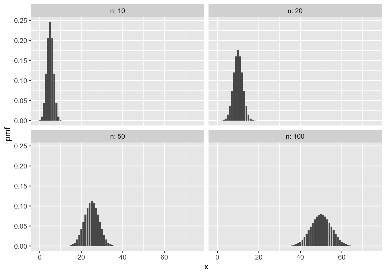
Here are some with \(n = 100\) and various \(p\).

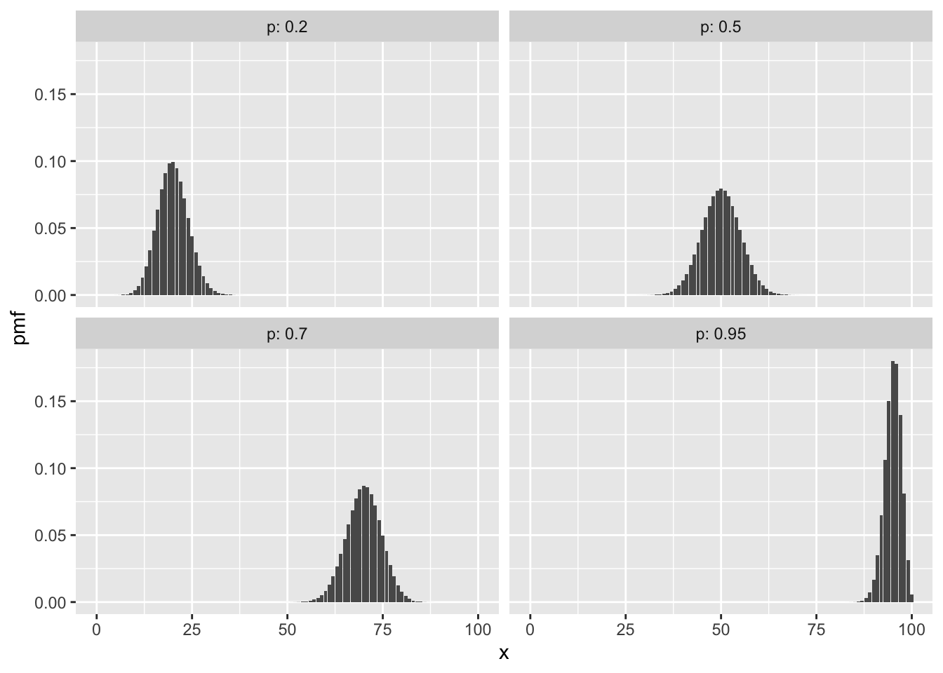
In these plots of binomial pmfs, the distributions are roughly balanced around a peak. The balancing point is the expected value of the random variable, which for binomial rvs is quite intuitive:

Theorem 5.4

Let \(X\) be a binomial random variable with \(n\) trials and probability of success \(p\). Then \[ E[X] = np \]

We will see a simple proof of this once we talk about the expected value of the sum of random variables. Here is a proof using the pmf and the definition of expected value directly.

Proof:

The binomial theorem says that: \[ (a + b)^n = a^n + {\binom{n}{1}}a^{n-1}b^1 + {\binom{n}{2}}a^{n-2}b^2 + \dotsb + {\binom{n}{n-1}}a^1 b^{n-1} + b^n \] Take the derivative of both sides with respect to \(a\): \[ n(a + b)^{n-1} = na^{n-1} + (n-1){\binom{n}{1}}a^{n-2}b^1 + (n-2){\binom{n}{2}}a^{n-3}b^2 + \dotsb + 1{\binom{n}{n-1}}a^0 b^{n-1} + 0 \] Multiply both sides by \(a\): \[ an(a + b)^{n-1} = na^{n} + (n-1){\binom{n}{1}}a^{n-1}b^1 + (n-2){\binom{n}{2}}a^{n-2}b^2 + \dotsb + 1{\binom{n}{n-1}}a^1 b^{n-1} + 0\] Finally, substitute \(a = p\), \(b = 1-p\), and note that \(a + b = 1\): \[ pn = np^{n} + (n-1){\binom{n}{1}}p^{n-1}(1-p)^1 + (n-2){\binom{n}{2}}p^{n-2}(1-p)^2 + \dotsb + 1{\binom{n}{n-1}}p^1 (1-p)^{n-1} + 0(1-p)^n \] or \[ pn = \sum_{x = 0}^{n} x {\binom{n}{x}}p^x(1-p)^{n-x} = E[X] \] Since for \(X \sim \text{Binom}(n,p)\), the pmf is given by \(P(X = x) = {\binom{n}{x}}p^{x}(1-p)^{n-x}\)

Example 5.20

Suppose 100 dice are thrown. What is the expected number of sixes? What is the probability of observing 10 or fewer sixes?

We assume that the results of the dice are independent and that the probability of rolling a six is \(p = 1/6\). The random variable \(X\) is the number of sixes observed, and \(X \sim \text{Binom}(100,1/6)\).

Then \(E[X] = 100 \cdot \frac{1}{6} \approx 16.67\). That is, we expect 1/6 of the 100 rolls to be a six.

The probability of observing 10 or fewer sixes is \[ P(X \le 10) = \sum_{j=0}^{10} P(X = j) = \sum_{j=0}^{10} {\binom{100}{j}}(1/6)^j(5/6)^{100-j} \approx 0.0427. \] In R,

sum(dbinom(0:10, 100, 1 / 6))

## [1] 0.04269568

R also provides the function pbinom, which is the cumulative sum of the pmf. The cumulative sum of a pmf is important enough that it gets its own name: the cumulative distribution function. We will say more about the cumulative distribution function in general in Section @ref{continuousrv}.

pbinom(x, size = n, prob = p) gives \(P(X \leq x)\) for \(X \sim \text{Binom}(n,p)\).

In the previous example, we could compute \(P(X \le 10)\) as

pbinom(10, 100, 1 / 6)

## [1] 0.04269568

Example 5.21

Suppose Alice and Bob are running for office, and 46% of all voters prefer Alice. A poll randomly selects 300 voters from a large population and asks their preference. What is the expected number of voters who will report a preference for Alice? What is the probability that the poll results suggest Alice will win?

Let “success” be a preference for Alice, and \(X\) be the random variable equal to the number of polled voters who prefer Alice. It is reasonable to assume that \(X \sim \text{Binom}(300,0.46)\) as long as our sample of 300 voters is a small portion of the population of all voters.

We expect that \(0.46 \cdot 300 = 138\) of the 300 voters will report a preference for Alice.

For the poll results to show Alice in the lead, we need \(X > 150\). To compute \(P(X > 150)\), we use \(P(X > 150) = 1 - P(X \leq 150)\) and then

1 - pbinom(150, 300, 0.46)

## [1] 0.07398045

There is about a 7.4% chance the poll will show Alice in the lead, despite her imminent defeat.

R provides the function rbinom to simulate binomial random variables. The first argument to rbinom is the number of random values to simulate, and the next arguments are size = n and prob = p. Here are 15 simulations of the Alice vs. Bob poll:

rbinom(15, size = 300, prob = 0.46)

##  [1] 132 116 129 139 165 137 138 142 134 140 140 134 134 126 149

In this series of simulated polls, Alice appears to be losing in all except the fifth poll where she was preferred by \(165/300 = 55\%\) of the selected voters.

We can compute \(P(X > 150)\) by simulation

X <- rbinom(10000, 300, 0.46)
mean(X > 150)

## [1] 0.0714

which is close to our theoretical result that Alice should appear to be winning 7.4% of the time.

Finally, we can estimate the expected number of people in our poll who say they will vote for Alice and compare that to the value of 138 that we calculated above.

mean(X) #estimate of expected value

## [1] 137.9337

3.3.2 Geometric

Definition 5.22

A random variable \(X\) is said to be a geometric random variable with parameter \(p\) if \[ P(X = x) = (1 - p)^{x} p, \qquad x = 0, 1,2, \ldots \]

Theorem 5.5

Let \(X\) be the random variable that counts the number of failures before the first success in a Bernoulli process with probability of success \(p\). Then \(X\) is a geometric random variable.

Proof:

The only way to achieve \(X = x\) is to have the first \(x\) trials result in failure and the next trial result in success. Each failure happens with probability \(1-p\), and the final success happens with probabilty \(p\). Since the trials are independent, we multiply \(1-p\) a total of \(x\) times, and then multiply by \(p\).

As a check, we show that the geometric pmf does sum to one. This requires summing an infinite geometric series: \[ \sum_{x=0}^{\infty} p(1-p)^x = p \sum_{x=0}^\infty (1-p)^x = p \frac{1}{1-(1-p)} = 1 \]

Alert 5.2

We defined the geometric random variable \(X\) so that it is compatible with functions built in to R. Some sources let \(Y\) be the number of trials required for the first success, and call \(Y\) geometric. In that case \(Y = X + 1\), as the final success counts as one additional trial.

The functions dgeom, pgeom and rgeom are available for working with a geometric random variable \(X \sim \text{Geom}(p)\):

• dgeom(x,p) is the pmf, and gives \(P(X = x)\)
• pgeom(x,p) gives \(P(X \leq x)\)
• rgeom(N,p) simulates \(N\) random values of \(X\).

Example 5.23

A die is tossed until the first 6 occurs. What is the probability that it takes 4 or more tosses?

We define success as a roll of six, and let \(X\) be the number of failures before the first success. Then \(X \sim \text{Geom}(1/6)\), a geometric random variable with probability of success \(1/6\).

Taking 4 or more tosses corresponds to the event \(X \geq 3\). Theoretically, \[ P(X \ge 3) = \sum_{x=3}^\infty P(X = x) = \sum_{x=3}^\infty \frac{1}{6}\cdot\left(\frac{5}{6}\right)^x = \frac{125}{216} \approx 0.58. \] We cannot perform the infinite sum with dgeom, but we can come close by summing to a large value of \(x\):

sum(dgeom(3:1000, 1 / 6))

## [1] 0.5787037

Another approach is to apply rules of probability to see that \(P(X \ge 3) = 1 - P(X < 3)\) Since \(X\) is discrete, \(X < 3\) and \(X \leq 2\) are the same event. Then \(P(X \ge 3) = 1 - P(X \le 2)\):

1 - sum(dgeom(0:2, 1 / 6))

## [1] 0.5787037

Rather than summing the pmf, we may use pgeom:

1 - pgeom(2, 1 / 6)

## [1] 0.5787037

The function pgeom has an option lower.tail=FALSE which makes it compute \(P(X > x)\) rather than \(P(X \le x)\), leading to maybe the most concise method:

pgeom(2, 1 / 6, lower.tail = FALSE)

## [1] 0.5787037

Finally, we can use simulation to approximate the result:

X <- rgeom(10000, 1 / 6)
mean(X >= 3)

## [1] 0.581

All of these show there is about a 0.58 probability that it will take four or more tosses to roll a six.

Here are some plots of geometric pmfs with various \(p\).

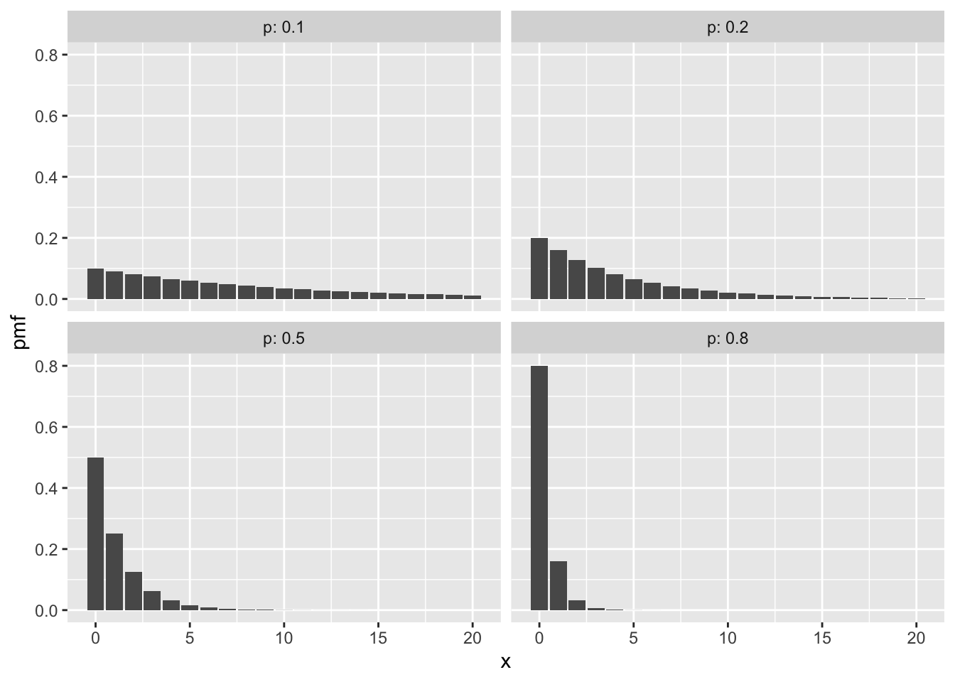
Observe that for smaller \(p\), we see that \(X\) is likely to be larger. The lower the probability of success, the more failures we expect before our first success.

Theorem 5.6

Let \(X\) be a geometric random variable with probability of success \(p\). Then \[ E[X] = \frac{(1-p)}{p} \]

Proof:

Let \(X\) be a geometric rv with success probability \(p\). Let \(q = 1-p\) be the failure probability. We must compute \(E[X] = \sum_{x = 0}^\infty x pq^x\). Begin with a geometric series in \(q\): \[ \sum_{x = 0}^\infty q^x = \frac{1}{1-q} \] Take the derivative of both sides with respect to \(q\): \[ \sum_{x = 0}^\infty xq^{x-1} = \frac{1}{(1-q)^2} \] Multiply both sides by \(pq\): \[ \sum_{x = 0}^\infty xpq^x = \frac{pq}{(1-q)^2} \] Replace \(1-q\) with \(p\) and we have shown: \[ E[X] = \frac{q}{p} = \frac{1-p}{p} \]

Example 5.24

Roll a die until a six is tossed. What is the expected number of rolls?

The expected number of failures is given by \(X \sim \text{Geom}(1/6)\), and so we expect \(\frac{5/6}{1/6} = 5\) failures before the first success. Since the number of total rolls is one more than the number of failures, we expect 6 rolls, on average, to get a six.

Example 5.25

Professional basketball player Steve Nash was a 90% free throw shooter over his career. If Steve Nash starts shooting free throws, how many would he expect to make before missing one? What is the probability that he could make 20 in a row?

Let \(X\) be the random variable which counts the number of free throws Steve Nash makes before missing one. We model a Steve Nash free throw as a Bernoulli trial, but we choose “success” to be a missed free throw, so that \(p = 0.1\) and \(X \sim \text{Geom}(0.1)\). The expected number of “failures” is \(E[X] = \frac{0.9}{0.1} = 9\), which means we expect Steve to make 9 free throws before missing one.

To make 20 in a row requires \(X \ge 20\). Using \(P(X \ge 20) = 1 - P(X \le 19)\),

1 - pgeom(19, 0.1)

## [1] 0.1215767

we see that Steve Nash could run off 20 (or more) free throws in a row about 12% of the times he wants to try.

3.4 Continuous random variables

Definition 5.26

A probability density function (pdf) is a function \(f\) such that:

1. \(f(x) \ge 0\) for all \(x\).
2. \(\int f(x)\, dx = 1\).

Definition 5.27

A continuous random variable \(X\) is a random variable described by a probability density function, in the sense that: \[ P(a \le X \le b) = \int_a^b f(x)\, dx. \] whenever \(a \le b\), including the cases \(a = -\infty\) or \(b = \infty\).

Definition 5.28

The cumulative distribution function (cdf) associated with \(X\) (either discrete or continuous) is the function \(F(x) = P(X \le x)\), or written out in terms of pdf’s and cdf’s:

\[ F(x) = P(X \le x) = \begin{cases} \int_{-\infty}^x f(t)\, dt& X \text{ is continuous}\\ \sum_{n = -\infty}^x p(n) & X \text{ is discrete} \end{cases} \]

By the Fundamental Theorem of Calculus, when \(X\) is continuous, \(F\) is a continuous function, hence the name continuous rv. The function \(F\) is sometimes referred to as the distribution function of \(X\).

One major difference between discrete rvs and continuous rvs is that discrete rv’s can take on only countably many different values, while continuous rvs typically take on values in an interval such as \([0,1]\) or \((-\infty, \infty)\).

Theorem 5.7

Let \(X\) be a continuous random variable with pdf \(f\) and cdf \(F\).

1. \(\frac{d}{dx} F = f\).
2. \(P(a \le X \le b) = F(b) - F(a)\)
3. \(P(X \ge a) = 1 - F(a) = \int_a^\infty f(x)\, dx\)

Proof:

All of these follow directly from the Fundamental Theorem of Calculus.

Alert 5.3

For a continous rv \(X\), the probability \(P(X = x)\) is always zero, for any \(x\). Therefore, \(P(X \ge a) = P(X > a)\) and \(P(X \le b) = P(X < b)\).

Example 5.29

Suppose that \(X\) has pdf \(f(x) = e^{-x}\) for \(x > 0\), as graphed below.

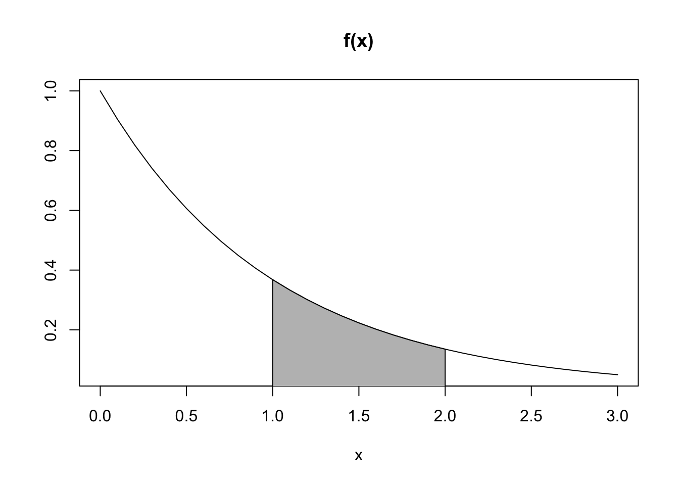
1. Find \(P(1 \le X \le 2)\), which is the shaded area shown in the graph. By definition, \[ P(1\le X \le 2) = \int_1^2 e^{-x}\, dx = -e^{-x}\Bigl|_1^2 = e^{-1} - e^{-2} \approx .233 \]

2. Find \(P(X \ge 1| X \le 2)\). This is the conditional probability that \(X\) is greater than 1, given that \(X\) is less than or equal to 2. We have \[\begin{align*} P(X \ge 1| X \le 2) &= P( X \ge 1 \cap X \le 2)/P(X \le 2)\\ &=P(1 \le X \le 2)/P(X \le 2)\\ &=\frac{e^{-1} - e^{-2}}{1 - e^{-2}} \approx .269 \end{align*}\]

Let \(X\) have the pdf: \[ f(x) = \begin{cases} 0 & x < 0\\ 1 & 0 \le x \le 1\\ 0 & x \ge 1 \end{cases} \]

\(X\) is called the uniform random variable on the interval \([0,1]\), and realizes the idea of choosing a random number between 0 and 1.

Here are some simple probability computations involving \(X\): \[ \begin{aligned} P(X > 0.3) &= \int_{0.3}^{1}1\,dx = 0.7\\ \\ P(0.2 < X < 0.5) &= \int_{0.2}^{0.5}1\,dx = 0.3 \end{aligned} \]

The cdf for \(X\) is given by: \[ F(x) = \begin{cases} 0 & x < 0\\ x & 0\le x \le 1\\ 1 & x \ge 1 \end{cases} \]

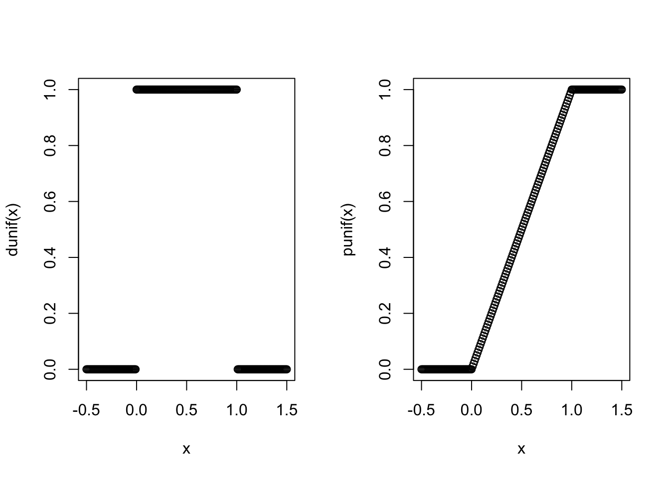
The pdf and cdf of \(X\) are implemented in R with the functions dunif and punif. Here are plots of these functions:

x <- seq(-0.5, 1.5, 0.01)
plot(x, dunif(x))
plot(x, punif(x))

We can produce simulated values of \(X\) with the function runif, and use those to estimate probabilities:

X <- runif(10000)
mean(X > 0.3)

## [1] 0.7041

mean(0.2 < X & X < 0.5)

## [1] 0.3015

Here, we have used the vectorized version of the and operator, &.

Alert 5.4

It is important to distinguish between the operator & and the operator && when doing simulations, or any time that you are doing logical operations on vectors. If you use && on two vectors, then it ignores all of the values in each vector except the first one!

For example,

c(TRUE, TRUE, TRUE) && c(TRUE, FALSE, FALSE)

## [1] TRUE

But, compare to

c(TRUE, TRUE, TRUE) & c(TRUE, FALSE, FALSE)

## [1]  TRUE FALSE FALSE

Example 5.30

Suppose \(X\) is a random variable with cdf given by

\[ F(x) = \begin{cases} 0 & x < 0\\ x/2 & 0\le x \le 2\\ 1 & x \ge 2 \end{cases} \]

1. Find \(P(1 \le X \le 2)\). To do this, we note that \(P(1 \le X \le 2) = F(2) - F(1) = 1 - 1/2 = 1/2\).

2. Find \(P(X \ge 1/2)\). To do this, we note that \(P(X \ge 1/2) = 1 - F(1/2) = 1 - 1/4 = 3/4\).

3. To find the pdf associated with \(X\), we take the derivative of \(F\). Since pdf’s are only used via integration, it doesn’t matter how we define the pdf at the places where \(F\) is not differentiable. In this case, we set \(f\) equal to \(1/2\) at those places to get \[ f(x) = \begin{cases} 1/2 & 0 \le x \le 2\\ 0& \text{otherwise} \end{cases} \] This example is also a uniform random variable, this time on the interval \([0,2]\)

3.4.1 Expected value of a continuous random variable

Definition 5.31

Let \(X\) be a continuous random variable with pdf \(f\).

The expected value of \(X\) is \[ E[X] = \int_{-\infty}^{\infty} x f(x)\, dx \]

Example 5.32

Find the expected value of \(X\) when its pdf is given by \(f(x) = e^{-x}\) for \(x > 0\).

We compute \[ E[X] = \int_{-\infty}^{\infty}f(x) dx = \int_0^\infty x e^{-x} \, dx = \left(-xe^{-x} - e^{-x}\right)\Bigr|_0^\infty = 1 \] (Recall: to integrate \(xe^{-x}\) you use integration by parts)

Example 5.33

Find the expected value of the uniform random variable on \([0,1]\). Using integration, we get the exact result: \[ E[X] = \int_0^1 x \cdot 1\, dx = \frac{x^2}{2}\Biggr|_0^1 = \frac{1}{2} \]

Approximating with simulation,

X <- runif(10000)
mean(X)

## [1] 0.5024951

Remark

Observe that the formula for the expected value of a continous rv is the same as the formula for center of mass. If the area under the pdf \(f(x)\) is cut from a thin sheet of material, the expected value is the point on the \(x\)-axis where this material would balance.

The balance point is at \(X = 1/2\) for the uniform random variable on [0,1], since the pdf describes a square with base \([0,1]\).

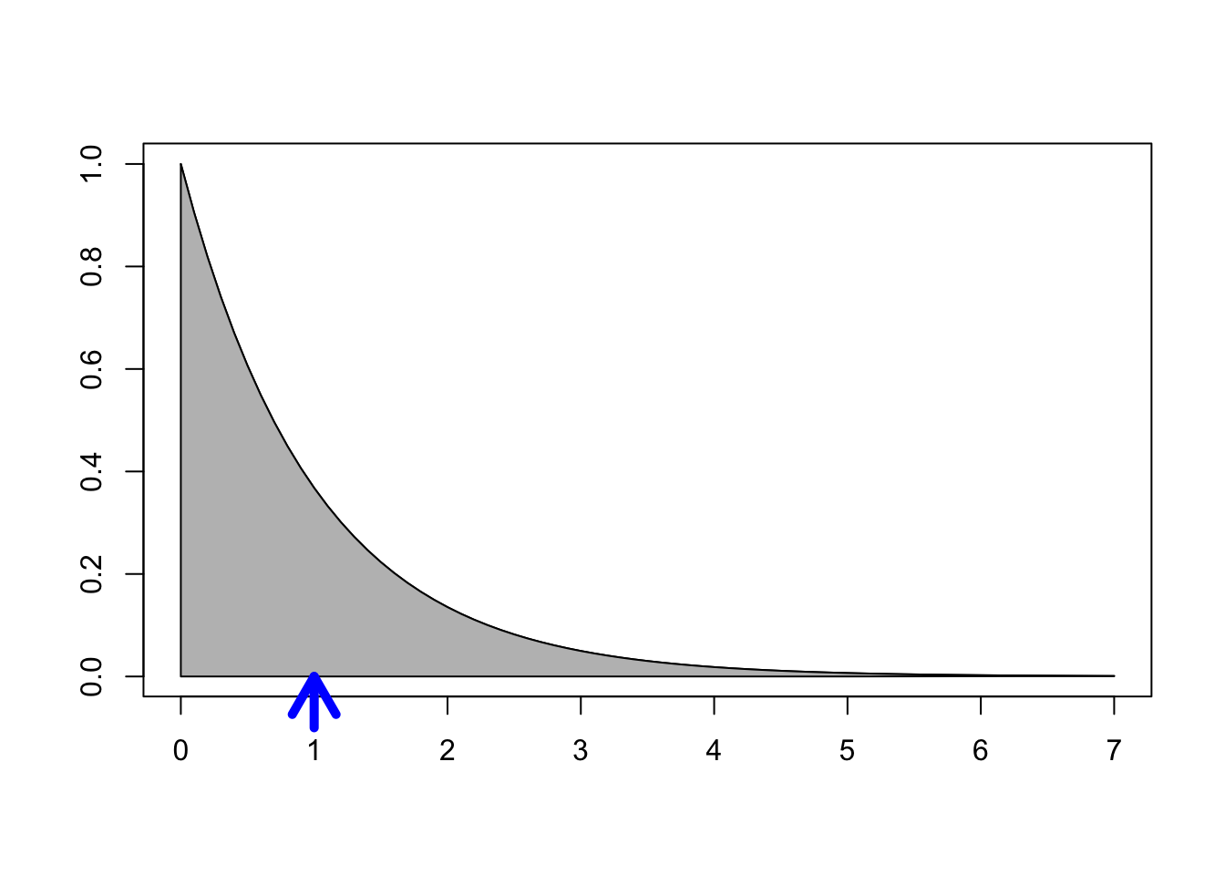
For \(X\) with pdf \(f(x) = e^{-x}, x \ge 0\), the picture below shows \(E[X]=1\) as the balancing point for the shaded region:

3.5 Functions of a random variable

Recall that a random variable \(X\) is a function from the sample space \(S\) to \(\mathbb{R}\). Given a function \(g : \mathbb{R} \to \mathbb{R},\) we can form the random variable \(g \circ X\), usually written \(g(X)\).

For example, suppose we have a new technique for measuring the length of an object. In order to assess the accuracy of the new technique, we might find an object of known length \(\mu\), and measure it multiple times using the new technique. If \(X\) is the length as measured by the new technique, we might be more interested in the error \(X - \mu\) or the absolute error \(|X - \mu|\) of the measurement than we are in \(X\), the value of the measurement.

As another example, if \(X\) is the value from a six-sided die roll and \(g(x) = x^2\), then \(g(X) = X^2\) is the value of a single six-sided die roll, squared. Here \(X^2\) can take the values \(1, 4, 9, 16, 25, 36\), all equally likely.

The distribution of \(g(X)\) can be difficult to compute. However, we can often understand \(g(X)\) by using the pdf of \(X\) itself. The most important situation for our purposes is to compute the expected value, \(E[g(x)]\):

\[ E\left[g(X)\right] = \begin{cases} \sum g(x) p(x) & X {\rm \ \ discrete} \\ \int g(x) f(x)\, dx & X {\rm \ \ continuous}\end{cases} \]

Example 5.34

Let \(X\) be the value of a six-sided die roll. Then \[ E[X^2] = 1^2\cdot 1/6 + 2^2\cdot 1/6 + 3^2\cdot 1/6 + 4^2\cdot 1/6 + 5^2\cdot 1/6 + 6^2\cdot 1/6 = 91/6 \approx 15.17\] Computing with simulation is straightforward:

X <- sample(1:6, 10000, replace = TRUE)
mean(X^2)

## [1] 15.0689

Example 5.35

Let \(X \sim \text{Binom}(3,0.5)\). Compute the expected value of \((X-1.5)^2\). Here \(X\) is discrete with pmf \(p(x) = {\binom{3}{x}} (.5)^3\) for \(x = 0,1,2,3\). We compute \[ \begin{split} E[(X-1.5)^2] &= \sum_{x=0}^3(x-1.5)^2p(x)\\ &= (0-1.5)^2\cdot 0.125 + (1-1.5)^2 \cdot 0.375 + (2-1.5)^2 \cdot 0.375 + (3-1.5)^2 \cdot 0.125\\ &= 0.75 \end{split} \] Since dbinom gives the pdf for binomial rvs, we can perform this exact computation in R:

x <- 0:3
sum((x - 1.5)^2 * dbinom(x, 3, 0.5))

## [1] 0.75

Example 5.36

Let \(X\) be the uniform random variable on \([0,1]\), and let \(Y = 1/X\).

What is \(P(Y < 3)\)? The event \(Y < 3\) is the same as \(1/X < 3\) or \(X > 1/3\), so \(P(Y < 3) = P(X > 1/3) = 2/3\). We can check with simulation:

X <- runif(10000)
Y <- 1 / X
mean(Y < 3)

## [1] 0.6619

On the other hand, the expected value of \(Y = 1/X\) is not well behaved. We compute: \[ E[1/X] = \int_0^1 \frac{1}{x} dx = \ln(x)\Bigr|_0^1 = \infty \] Small values of \(X\) are common enough that the huge values of \(1/X\) produced cause the expected value to be infinite. Let’s see what this does to simulations:

X <- runif(100)
mean(1 / X)

## [1] 4.116572

X <- runif(10000)
mean(1 / X)

## [1] 10.65163

X <- runif(1000000)
mean(1 / X)

## [1] 22.27425

Because the expected value is infinite, the simulations are not approaching a finite number as the size of the simulation increases. The reader is encouraged to try running these simulations multiple times to observe the inconsistency of the results.

Example 5.37

Compute \(E[X^2]\) for \(X\) that has pdf \(f(x) = e^{-x}\), \(x > 0\).

Using integration by parts: \[ E[X^2] = \int_0^\infty x^2 e^{-x}\, dx = \left(-x^2 e^{-x} - 2x e^{-x} - 2 e^{-x}\right)\Bigl|_0^\infty = 2. \]

We conclude this section with two simple but important observations about expected values. First, that expected value is linear. Second, that the expected value of a constant is that constant. Stated precisely:

Theorem 5.8

For random variables \(X\) and \(Y\), and constants \(a\), \(b\), and \(c\):

1. \(E[aX + bY] = aE[X] + bE[Y]\)
2. \(E[c] = c\)

The proofs follow from the definition of expected value and the linearity of integration and summation, and are left as exercises for the reader. With these theorems in hand, we can provide a much simpler proof for the formula of the expected value of a binomial random variable.

Let \(X \sim \text{Binom}(n, p)\). Then \(X\) is the number of successes in \(n\) Bernoulli trials, each with probability \(p\). Let \(X_1, \ldots, X_n\) be independent Bernoulli random variables with probability of success \(p\). That is, \(P(X_i = 1) = p\) and \(P(X_i = 0) = 1 - p\). It follows that \(X = \sum_{i = 1}^n X_i\). Therefore,

\[\begin{align*} E[X] &= E[\sum_{i = 1}^n X_i]\\ &= \sum_{i = 1}^n E[X_i] = \sum_{i = 1}^n p = np. \end{align*}\]

3.6 Variance and standard deviation

The variance of a random variable measures the spread of the variable around its expected value. Rvs with large variance can be quite far from their expected values, while rvs with small variance stay near their expected value. The standard deviation is simply the square root of the variance. The standard deviation also measures spread, but in more natural units which match the units of the random variable itself.

Definition 5.38

Let \(X\) be a random variable with expected value \(\mu = E[X]\). The variance of \(X\) is defined as \[ \text{Var}(X) = E[(X - \mu)^2] \] The standard deviation of \(X\) is written \(\sigma(X)\) and is the square root of the variance: \[ \sigma(X) = \sqrt{\text{Var}(X)} \]

Note that the variance of an rv is always positive (in the French sense¹¹), as it is the integral or sum of a positive function.

The next theorem gives a formula for the variance that is often easier than the definition when performing computations.

Theorem 5.9

\({\rm Var}(X) = E[X^2] - E[X]^2\)

Proof:

Applying linearity of expected values (Theorem 5.8) to the definition of variance yields: \[ \begin{split} E[(X - \mu)^2] &= E[X^2 - 2\mu X + \mu^2]\\ &= E[X^2] - 2\mu E[X] + \mu^2 = E[X^2] - 2\mu^2 + \mu^2\\ &= E[X^2] - \mu^2, \end{split} \] as desired.

Example 5.39

Let \(X \sim \text{Binom}(3,0.5)\). Here \(\mu = E[X] = 1.5\). In Example 5.35, we saw that \(E[(X-1.5)^2] = 0.75\). Then \(\text{Var}(X) = 0.75\) and the standard deviation is \(\sigma(X) = \sqrt{0.75} \approx 0.866\). We can check both of these using simulation and the built in R functions var and sd:

X <- rbinom(10000, 3, 0.5)
var(X)

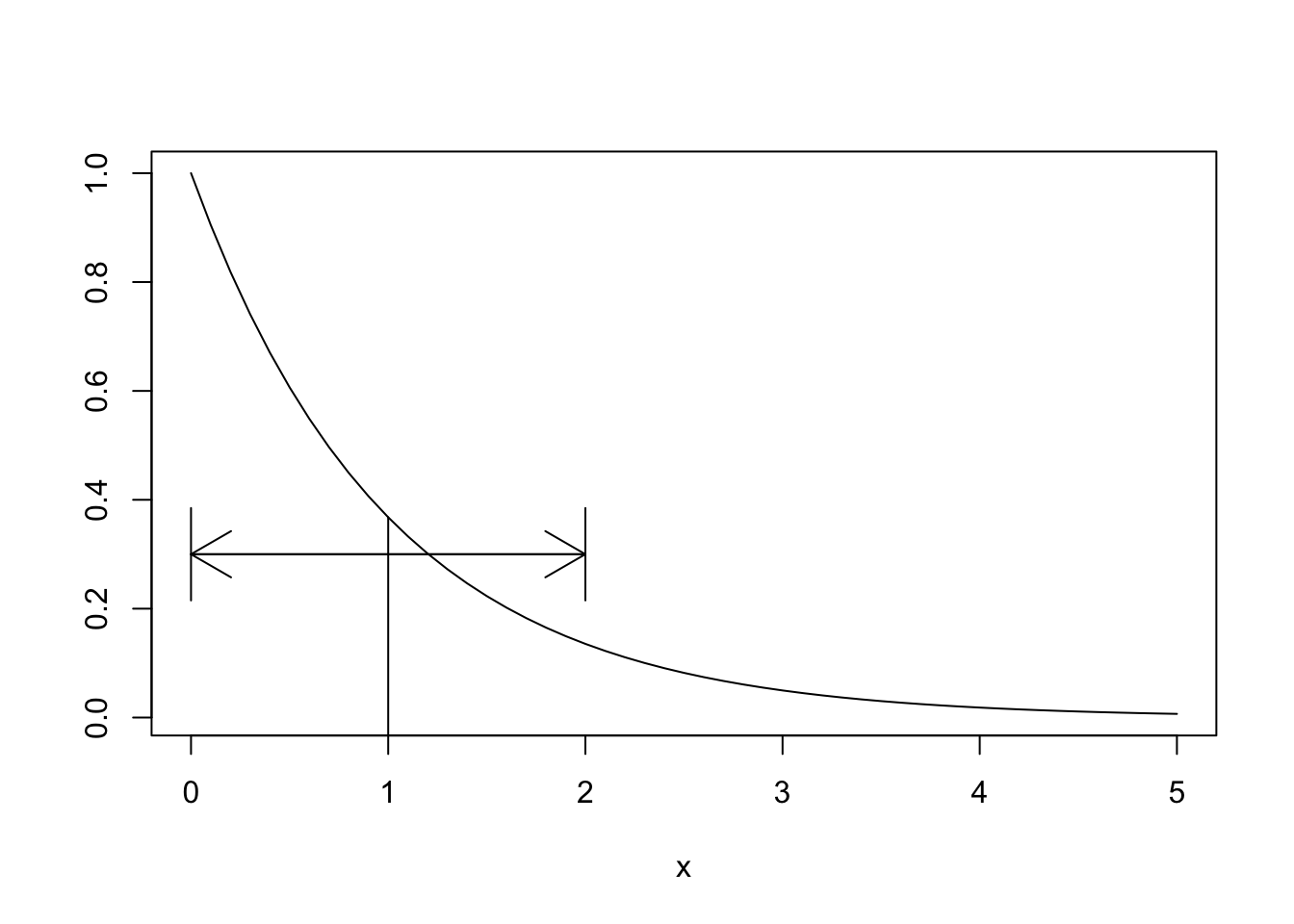
## [1] 0.7570209

sd(X)

## [1] 0.8700695

Example 5.40

Compute the variance of \(X\) if the pdf of \(X\) is given by \(f(x) = e^{-x}\), \(x > 0\).

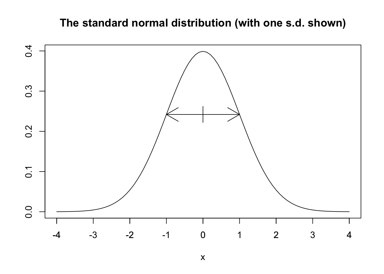
We have already seen that \(E[X] = 1\) and \(E[X^2] = 2\) (Example 5.37). Therefore, the variance of \(X\) is \[ \text{Var}(X) = E[X^2] - E[X]^2 = 2 - 1 = 1. \] The standard deviation \(\sigma(X) = \sqrt{1} = 1\). We interpret of the standard deviation \(\sigma\) as a spread around the mean, as shown in this picture:

Example 5.41

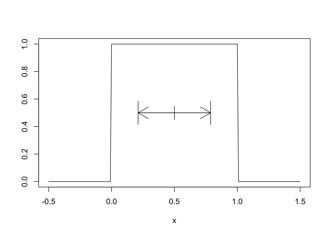
Compute the standard deviation of the uniform random variable \(X\) on \([0,1]\). \[ \begin{split} \text{Var}(X) &= E[X^2] - E[X]^2 = \int_0^1x^2 \cdot 1\, dx - \left(\frac{1}{2}\right)^2\\ &= \frac{1}{3} - \frac{1}{4} = \frac{1}{12} \approx 0.083. \end{split} \] So the standard deviation is \(\sigma(X) = \sqrt{1/12} \approx 0.289\). Shown as a spread around the mean of 1/2:

For many distributions, most of the values will lie within one standard deviation of the mean, i.e. within the spread shown in the example pictures. Almost all of the values will lie within 2 standard deviations of the mean. What do we mean by “almost all”? Well, 85% would be almost all. 15% would not be almost all. This is a very vague rule of thumb. Chebychev’s Theorem is a more precise statement. It says in particular that the probability of being more than 2 standard deviations away from the mean is at most 25%.

Sometimes, you know that the data you collect will likely fall in a certain range of values. For example, if you are measuring the height in inches of 100 randomly selected adult males, you would be able to guess that your data will very likely lie in the interval 60-84. You can get a rough estimate of the standard deviation by taking the expected range of values and dividing by 6; in this case it would be 24/6 = 4. Here, we are using the heuristic that it is very rare for data to fall more than three standard deviations from the mean. This can be useful as a quick check on your computations.

Unlike expected value, variance and standard deviation are not linear. However, variance and standard deviation do have scaling properties, and variance does distribute over sums in the special case of independent random variables:

Theorem 5.10

1. Let \(X\) be a rv and \(c\) a constant. Then \[ \begin{aligned} \text{Var}(cX) &= c^2\text{Var}(X)\\ \sigma(cX) &= c \sigma(X) \end{aligned} \]

2. Let \(X\) and \(Y\) be independent random variables. Then \[ {\rm Var}(aX + bY) = a^2 {\rm Var}(X) + b^2 {\rm Var}(Y) \]

Proof:

We prove part 1 here, and verify part 2 through simulation in Exercise 5.37. \[\begin{align*} {\rm Var}(cX) =& E[(cX)^2] - E[cX]^2 = c^2E[X^2] - (cE[X])^2\\ =&c^2\bigl(E[X^2] - E[X]^2) = c^2{\rm Var}(X) \end{align*}\]

Alert 5.5

1. Theorem 5.10 part 2 is only true when \(X\) and \(Y\) are independent.

2. If \(X\) and \(Y\) are independent, then \({\rm Var}(X - Y) = {\rm Var}(X) + {\rm Var}(Y)\).

Example 5.42 (The variance of a binomial random variable)

Let \(X \sim \text{Binom}(n, p)\). We have seen that \(X = \sum_{i = 1}^n X_i\), where \(X_i\) are independent Bernoulli random variables. Therefore,

\[\begin{align*} {\text {Var}}(X) &= {\text {Var}}(\sum_{i = 1}^n X_i)\\ &= \sum_{i = 1}^n {\text {Var}}(X_i) \\ &= \sum_{i = 1}^n p(1 - p) = np(1-p) \end{align*}\] where we have used that the variance of a Bernoulli random variable is \(p(1- p)\). Indeed, \(E[X_i^2] -E[X_i]^2 = p - p^2 = p(1 - p)\).

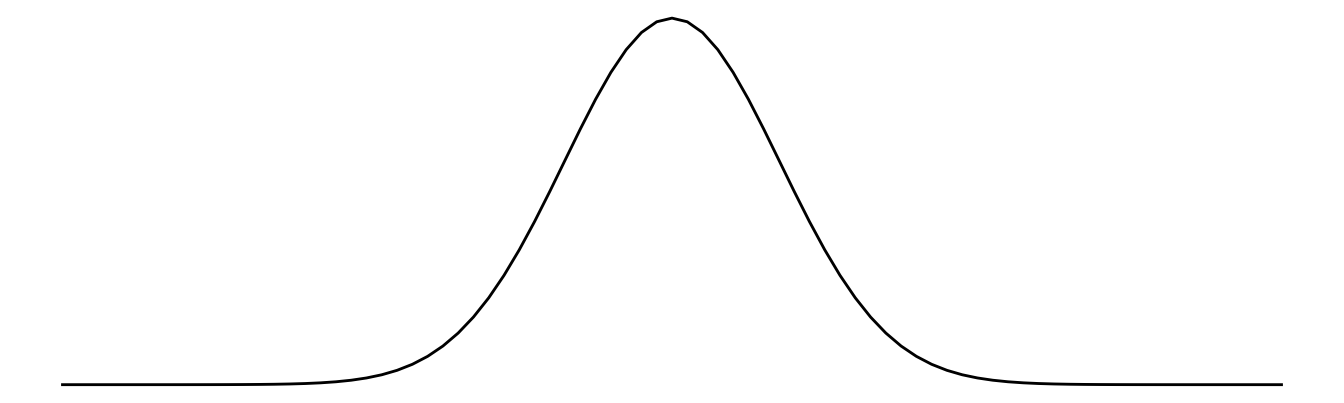
3.7 Normal random variables

The normal distribution is the most important in statistics. It is often referred to as the bell curve, because its shape resembles a bell:

The importance of the normal distribution stems from the Central Limit Theorem, which (very loosely) states that many random variables have normal distributions. A little more accurately, the Central Limit Theorem says that random variables which are affected by many small independent factors are approximately normal.

For example, we might model the heights of adult females with a normal distribution. We imagine that adult height is affected by genetic contributions from generations of parents together with the sum of contributions from food eaten and other environmental factors. This is a reason to try a normal model for heights of adult females, and certainly should not be seen as a theoretical justification of any sort that adult female heights must be normal.

Many measured quantities are commonly modeled with normal distributions. Biometric measurements (height, weight, blood pressure, wingspan) are often nearly normal. Standardized test scores, economic indicators, scientific measurement errors, and variation in manufacturing processes are other examples.

The mathematical definition of the normal distribution begins with the function \(h(x) = e^{-x^2}\), which produces the bell shaped curve shown above, centered at zero and with tails that decay very quickly to zero. By itself, \(h(x) = e^{-x^2}\) is not a distribution since it does not have area 1 underneath the curve. In fact:

\[ \int_{-\infty}^\infty e^{-x^2} dx = \sqrt{\pi} \]

This famous result is known as the Gaussian integral. Its proof is left to the reader in Exercise ??.3. By rescaling we arrive at an actual pdf given by \(g(x) = \frac{1}{\sqrt{\pi}}e^{-x^2}\). The distribution \(g(x)\) has mean zero and standard deviation \(\frac{1}{\sqrt{2}} \approx 0.707\). The inflection points of \(g(x)\) are also at \(\pm \frac{1}{\sqrt{2}}\) and so rescaling by 2 in the \(x\) direction produces a pdf with standard deviation 1 and inflection points at \(\pm 1\).

Definition 5.43

The standard normal random variable \(Z\) has probability density function given by \[ f(x) = \frac{1}{\sqrt{2\pi}} e^{-x^2/2} \]

The R function pnorm computes the cdf of the normal distribution, as pnorm(x) \(= P(Z \leq x)\). Using pnorm, we can compute the probability that \(Z\) lies within 1, 2, and 3 standard deviations of its mean:

• \(P(-1 \leq Z \leq 1) = P(Z \leq 1) - P(Z \leq -1) =\) pnorm(1) - pnorm(-1) = 0.6826895.
• \(P(-2 \leq Z \leq 2) = P(Z \leq 2) - P(Z \leq -2) =\) pnorm(2) - pnorm(-2) = 0.9544997.
• \(P(-3 \leq Z \leq 3) = P(Z \leq 3) - P(Z \leq -3) =\) pnorm(3) - pnorm(-3) = 0.9973002.

By shifting and rescaling \(Z\), we define the normal random variable with mean \(\mu\) and standard deviation \(\sigma\):

Definition 5.44

The normal random variable \(X\) with mean \(\mu\) and standard deviation \(\sigma\) is given by \[ X = \sigma Z + \mu. \] We write \(X \sim \text{Normal}(\mu,\sigma)\).

The pdf of a normal random variable is given in the following theorem.

Theorem 5.11

Let \(X\) be a normal random variable with parameters \(\sigma\) and \(\mu\). The probability mass function of \(X\) is given by \[ f(x) = \frac {1}{\sqrt{2pi}\sigma} e^{-(x - \mu)^2/(2\sigma^2)} \qquad -\infty < x < \infty \]

The parameter names are the mean \(\mu\) and the standard deviation \(\sigma\).

For any normal random variable, approximately:

• 68% of the normal distribution lies within 1 standard deviation of the mean.
• 95% lies within two standard deviations of the mean.
• 99.7% lies within three standard deviations of the mean.

This fact is sometimes called the empirical rule.

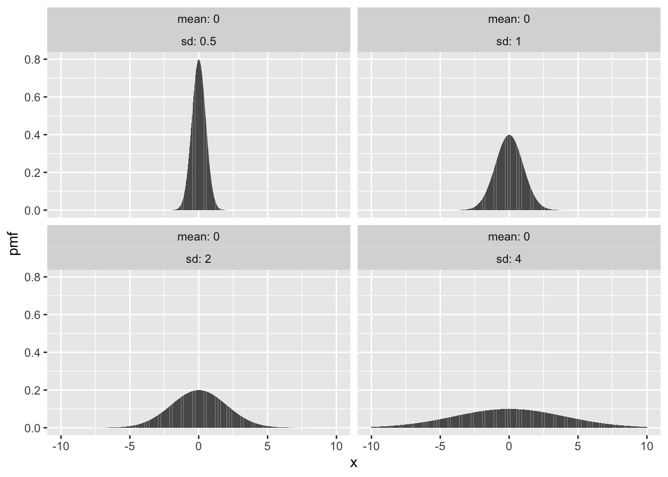
Here are some examples of normal distributions with fixed mean \(\mu = 0\) and various values of the standard deviation \(\sigma\):

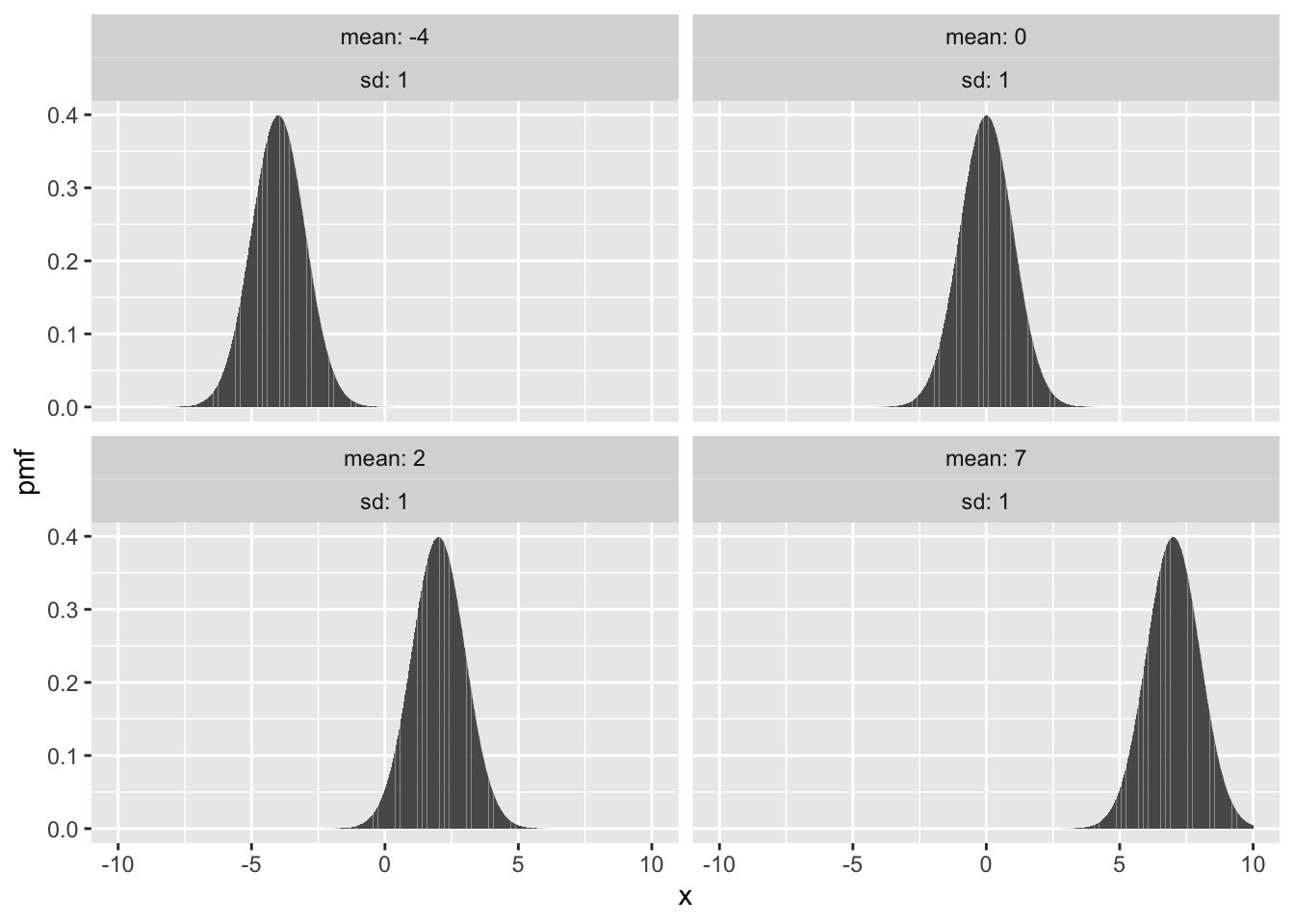
Here are normal distributions with fixed standard deviation \(\sigma = 1\) and various means \(\mu\):

3.7.1 Computations with normal random variables

R has built in functions for working with normal distributions and normal random variables. The root name for these functions is norm, and as with other distributions the prefixes d,p, and r specify the pdf, cdf, or random sampling. If \(X \sim \text{Normal}(\mu,\sigma)\):

• dnorm(x,mu,sigma) gives the height of the pdf at \(x\).
• pnorm(x,mu,sigma) gives \(P(X \leq x)\), the cdf.
• qnorm(p,mu,sigma) gives the value of \(x\) so that \(P(X \leq x) = p\), which is the inverse cdf.
• rnorm(N,mu,sigma) simulates \(N\) random values of \(X\).

Here are some simple examples:

Example 5.45

Let \(X \sim {\rm Normal}(\mu = 3, \sigma = 2)\). Find \(P(X \le 4)\) and \(P(0 \le X \le 5)\).

pnorm(4, mean = 3, sd = 2)

## [1] 0.6914625

pnorm(5, 3, 2) - pnorm(0, 3, 2)

## [1] 0.7745375

Example 5.46

Let \(X \sim {\rm Normal}(100,30)\). Find the value of \(q\) such that \(P(X \le q) = 0.75\). One approach is to try various choices of \(q\) until discovering that pnorm(120,100,30) is close to 0.75. However, the purpose of the qnorm function is to answer this exact question:

qnorm(0.75, 100, 30)

## [1] 120.2347

Example 5.47

The length of dog pregnancies from conception to birth varies according to a distribution that is approximately normal with mean 63 days and standard deviation 2 days.

1. What percentage of dog pregnancies last 60 days or less?
2. What percentage of dog pregnancies last 67 days or more?
3. What range covers the shortest 90% of dog pregnancies?
4. What is the narrowest range of times that covers 90% of dog pregnancies?

We let \(X\) be the random variable which is the length of a dog pregnancy. We model \(X \sim \text{Normal}(63,2)\). Then parts a and b ask for \(P(X \leq 60)\) and \(P(X \geq 67)\) and we can compute these with pnorm as follows:

pnorm(60, 63, 2)

## [1] 0.0668072

1 - pnorm(67, 63, 2)

## [1] 0.02275013

For part c, we want \(x\) so that \(P(X \leq x) = 0.90\). This is qnorm(0.90,63,2)=65.6, so 90% of dog pregnancies are shorter than 65.6 days.

For part d, we need to use the fact that the pdf’s of normal random variables are symmetric about their mean, and decreasing away from the mean. So, if we want the shortest interval that contains 90% of dog pregnancies, it should be centered at the mean with 5% of pregnancies to the left of the interval, and 5% of the pregnancies to the right of the interval. We get an interval of the form [qnorm(0.05, 63, 2), qnorm(0.95, 63, 2)], or approximately [59.7, 66.3]. The length of this interval is 6.6, which is much smaller than the length of the interval in the interval computed in c, which was 65.6.

Example 5.48

Let \(Z\) be a standard normal random variable. Find the mean and standard deviation of the variable \(e^Z\).

We solve this with simulation:

Z <- rnorm(100000, 0, 1)
mean(exp(Z))

## [1] 1.645643

sd(exp(Z))

## [1] 2.139868

The mean of \(e^Z\) is approximately 1.6, and the standard deviation is approximately 2.1. Note that even with 100000 simulated values these answers are not particularly accurate because on rare occasions \(e^Z\) takes on very large values.

Example 5.49

Suppose you are picking seven women at random from a university to form a starting line-up in an ultimate frisbee game. Assume that the women’s heights at this university are normally distributed with mean 64.5 inches (5 foot, 4.5 inches) and standard deviation 2.25 inches. What is the probability that 3 or more of the women are 68 inches (5 foot, 8 inches) or taller?

To do this, we first determine the probability that a single randomly selected woman is 68 inches or taller. Let \(X\) be a normal random variable with mean 64 and standard deviation 2.25. We compute \(P(X \ge 68)\) using pnorm:

pnorm(68, 65, 2.25, lower.tail = FALSE)

## [1] 0.09121122

Now, we need to compute the probability that 3 or more of the 7 women are 68 inches or taller. Since the population of all women at a university is much larger than 7, the number of women in the starting line-up who are 68 inches or taller is binomial with \(n = 7\) and \(p = 0.09121122\), which we computed in the previous step. We compute the probability that at least 3 are 68 inches as

sum(dbinom(3:7, 7, 0.09121122))

## [1] 0.02004754

So, there is about a 2 percent chance that at least three will be 68 inches or taller. Looking at the 2019 national champion UC San Diego Psychos roster, none of the players listed are 68 inches or taller, which has about a 50-50 chance of occurring according to our model.

Example 5.50

Throwing a dart at a dartboard with the bullseye at the origin, model the location of the dart with independent coordinates \(X \sim \text{Normal}(0,3)\) and \(Y \sim \text{Normal}(0,3)\) (both in inches). What is the expected distance from the bullseye?

The distance from the bullseye is given by the Euclidean distance formula \(d = \sqrt{X^2+ Y^2}\). We simulate the \(X\) and \(Y\) random variables and then compute the mean of \(d\):

X <- rnorm(10000, 0, 3)
Y <- rnorm(10000, 0, 3)
d <- sqrt(X^2 + Y^2)
mean(d)

## [1] 3.78152

We expect the dart to land about 3.8 inches from the bullseye, on average.

3.7.2 Normal approximation to the binomial

The value of a binomial random variable is the sum of many small, independent factors: the Bernoulli trials. A special case of the Central Limit Theorem is that a binomial random variable can be well approximated by a normal random variable.

First, we need to understand the standard deviation of a binomial random variable.

Theorem 5.12

Let \(X \sim \text{Binom}(n,p)\). The variance and standard deviation of \(X\) are given by: \[\begin{align} \text{var}(X) &= np(1-p)\\ \sigma(X) &= \sqrt{np(1-p)} \end{align}\]

The proof of this theorem was given in Example 5.42. There is also an instructive proof that is similar to the proof of Theorem 5.3, except that we take the derivative of the binomial theorem two times and compute \(E[X(X-1)]\). The result follows from \(E[X^2] = E[X(X-1)] + E[X]\) and Theorem 5.9.

Now the binomial rv \(X\) can be approximated by a random normal variable with the same mean and standard deviation as \(X\):

Theorem 5.13

Fix \(p\). For large \(n\), the binomial random variable \(X \sim \text{Binom}(n,p)\) is approximately normal with mean \(np\) and standard deviation \(np(1-p)\).

The size of \(n\) required to make the normal approximation accurate depends on the accuracy required and also depends on \(p\). Binomial distributions with \(p\) close to 0 or 1 are not as well approximated by the normal distribution as those with \(p\) near 1/2.

This normal approximation was traditionally used to work with binomial random variables, since calculating the binomial distribution exactly requires quite a bit of computation. Probabilities for the normal distribution were readily available in tables, and so easier to use. With R, the pbinom function makes it easy to work with binomial pmfs directly.

Example 5.51

Let \(X \sim \text{Binom}(300,0.46)\). Compute \(P(X > 150)\).

Computing exactly, \(P(X > 150) =\) 1 - pbinom(150,300,0.46) = 0.0740.

To use the normal approximation, we calculate that \(X\) has mean \(300 \cdot 0.46 = 138\) and standard deviation \(\sqrt{300\cdot0.46\cdot0.54} \approx 8.63\). Then \(P(X > 150) \approx\) 1 - pnorm(150,138,8.63) = 0.0822.

As an improvement, notice that the continuous normal variable can take values in between 150 and 151, but the discrete binomial variable cannot. To account for this, we use a continuity correction and assign each integer value of the binomial variable to the one-unit wide interval centered at that integer. Then 150 corresponds to the interval (145.5,150.5) and 151 corresponds to the interval (150.5,151.5). To approximate \(X > 150\), we want our normal random variable to be larger than 150.5. The normal approximation with continuity correction gives \(P(X > 150) \approx\) 1 - pnorm(150.5,138,8.63) = 0.0737, much closer to the actual value of 0.0740.

3.8 Other special random variables

In this section, we discuss other commonly occurring special types of random variable. Two of these (the uniform and exponential) have already shown up as earlier examples of continuous distributions.

3.8.1 Poisson and exponential random variables

A Poisson process models events that happen at random times. For example, radioactive decay is a Poisson process, where each emission of a radioactive particle is an event. Other examples modeled by Poisson process are meteor strikes on the surface of the moon, customers arriving at a store, hits on a web page, and car accidents on a given stretch of highway.

In this section, we will discuss two natural random variables attached to a Poisson process. The Poisson random variable is discrete, and can be used to model the number of events that happen in a fixed time period. The exponential random variable is continuous, and models the length of time for the next event to occur.

We begin by defining a Poisson process. Suppose events occur spread over time. The events form a Poisson process if they satisfy the following assumptions:

Assumptions 5.1 (for a Poisson process)

1. The probability of an event occurring in a time interval \([a,b]\) depends only on the length of the interval \([a,b]\).
2. If \([a,b]\) and \([c,d]\) are disjoint time intervals, then the probability that an event occurs in \([a,b]\) is independent of whether an event occurs in \([c,d]\). (That is, knowing that an event occurred in \([a,b]\) does not change the probability that an event occurs in \([c,d]\).)
3. Two events cannot happen at the same time. (Formally, we need to say something about the probability that two or more events happens in the interval \([a, a + h]\) as \(h\to 0\).)
4. The probability of an event occurring in a time interval \([a,a + h]\) is roughly \(\lambda h\), for some constant \(\lambda\).

Property 4 says that events occur at a certain rate, which is denoted by \(\lambda\).

3.8.1.1 Poisson

Definition 5.52

The random variable \(X\) is said to be a Poisson random variable with rate \(\lambda\) if the pmf of \(X\) is given by \[ p(x) = e^{-\lambda} \frac{\lambda^x}{x!} \qquad x = 0, 1, \ldots \] The parameter \(\lambda\) is required to be larger than 0. We write \(X \sim \text{Pois}(\lambda)\).

Theorem 5.14

Let \(X\) be the random variable that counts the number of occurences in a Poisson process with rate \(\lambda\) over one unit of time. Then \(X\) is a Poisson random variable with rate \(\lambda\).

Proof: (heuristic)

We have not stated Assumption 5.1.4 precisely enough for a formal proof, so this is only a heuristic argument.

Suppose we break up the time interval from 0 to 1 into \(n\) pieces of equal length. Let \(X_i\) be the number of events that happen in the \(i\)th interval. When \(n\) is big, \((X_i)_{i = 1}^n\) is approximately a sequence of \(n\) Bernoulli trials, each with probability of success \(\lambda/n\). Therefore, if we let \(Y_n\) be a binomial random variable with \(n\) trials and probability of success \(\lambda/n\), we have:

\[\begin{align*} P(X = x) &= P(\sum_{i = 1}^n X_i = x)\\ &\approx P(Y_n = x)\\ &= {\binom{n}{x}} (\lambda/n)^x (1 - \lambda/n)^{(n - x)} \\ &\approx \frac{n^x}{x!} \frac{1}{n^x} \lambda^x (1 - \lambda/n)^n\\ &\to \frac{\lambda^x}{x!}{e^{-\lambda}} \qquad {\text {as}} n\to \infty \end{align*}\]

The key to defining the Poisson process formally correctly is to ensure that the above computation is mathematically justified.

We leave the proof that \(\sum_x p(x) = 1\) as Exercise ??.4, along with the proof of the following Theorem.

Theorem 5.15

The mean and variance of a Poisson random variable are both \(\lambda\).

Though the proof of the mean and variance of a Poisson is an exercise, we can also give a heuristic argument. From above, a Poisson with rate \(\lambda\) is approximately a Binomial rv \(Y_n\) with \(n\) trials and probability of success \(\lambda/n\) when \(n\) is large. The mean of \(Y_n\) is \(n \times \lambda/n = \lambda\), and the variance is \(n (\lambda/n)(1 - \lambda/n) \to \lambda\) as \(n\to\infty\).

Here some plots of Poisson pmfs with various means \(\lambda\).

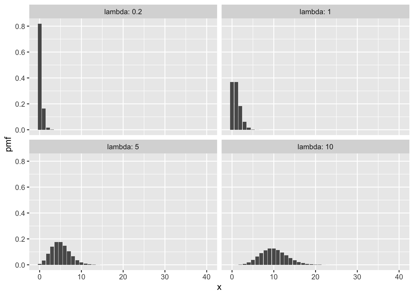
Observe in the plots that larger values of \(\lambda\) correspond to more spread-out distributions, since the standard deviation of a Poisson rv is \(\sqrt{\lambda}\). Also, for larger values of \(\lambda\), the Poisson distribution becomes approximately normal.

Example 5.53

The Taurids meteor shower is visible on clear nights in the Fall and can have visible meteor rates around five per hour. What is the probability that a viewer will observe exactly eight meteors in two hours?

We let \(X\) be the number of observed meteors in two hours, and model \(X \sim \text{Pois}(10)\), since we expect \(\lambda = 10\) meteors in our two hour time period. Computing exactly, \[ P(X = 8) = \frac{10^8}{8!}e^{-10} \approx 0.1126.\]

Using R, and the pdf dpois:

dpois(8, 10)

## [1] 0.112599

Or, by simulation with rpois:

meteors <- rpois(10000, 10)
mean(meteors == 8)

## [1] 0.1191

We find that the probability of seeing exactly 8 meteors is about 0.11.

Example 5.54

Suppose a typist makes typos at a rate of 3 typos per 10 pages. What is the probability that they will make at most one typo on a five page document?

We let \(X\) be the number of typos in a five page document. Assume that typos follow the properties of a Poisson rv. It is not clear that they follow it exactly. For example, if the typist has just made a mistake, it is possible that their fingers are no longer on home position, which means another mistake is likely soon after. This would violate the independence property (2) of a Poisson process. Nevertheless, modeling \(X\) as a Poisson rv is reasonable.

The rate at which typos occur per five pages is 1.5, so we use \(\lambda = 1.5\). Then we can compute \(P(X \leq 1) = \text{ppois}(1,1.5)=0.5578\). The typist has a 55.78% chance of making at most one typo on a five page document.

3.8.1.2 Exponential

Definition 5.55

An exponential random variable \(X\) with rate \(\lambda\) has pdf \[ f(x) = \lambda e^{-\lambda x}, \qquad x > 0 \]

Exponential rv’s measure the waiting time until the first event occurs in a Poisson process . The waiting time until an electronic component fails could be exponential. In a store, the time between customers could be modeled by an exponential random variable by starting the Poisson process at the moment the first customer enters.

Here are some plots of pdf’s with various rates.

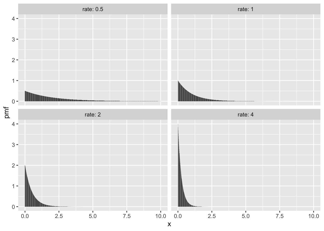
Observe from the pictures that the higher the rate, the smaller \(X\) will be. This is because we generally wait less time for events that occur more frequently.

Theorem 5.16

Let \(X \sim \text{Exp}(\lambda)\) be an exponential random variable with rate \(\lambda\). Then the mean and variance of \(X\) are: \[\begin{align} E[X] &= \frac{1}{\lambda}\\ \text{var}(X) &= \frac{1}{\lambda^2} \end{align}\]

Proof:

We compute the mean of an exponential random variable with rate \(\lambda\) using integration by parts as follows: \[\begin{align*} E[X]&=\int_{-\infty}^\infty x f(x)\, dx\\ &=\int_0^\infty x \lambda e^{-\lambda x} + \int_{-\infty}^0 x \cdot 0 \, dx\\ &= -xe^{-\lambda x} - \frac {1}{\lambda} e^{-\lambda x}\big|_{x = 0}^{x = \infty}\\ & = \frac {1}{\lambda} \end{align*}\]

For the variance, we compute the rather challenging integral: \[ E[X^2] = \int_0^\infty x^2 \lambda e^{-\lambda x} dx = \frac{2}{\lambda^2} \] Then \[ \text{var}(X) = E[X^2] - E[X]^2 = \frac{2}{\lambda^2} - \left(\frac{1}{\lambda}\right)^2 = \frac{1}{\lambda^2}. \]

Example 5.56

When watching the Taurids meteor shower, meteors arrive at a rate of five per hour. How long do you expect to wait for the first meteor? How long should you wait to have a 95% change of seeing a meteor?

Here, \(X\) is the length of time before the first meteor. We model the meteors as a Poisson process with rate \(\lambda = 5\) (and time in hours). Then \(E[X] = \frac{1}{5} = 0.2\) hours, or 12 minutes.

For a 95% chance, we are interested in finding \(x\) so that \(P(X < x) = 0.95\). One way to approach this is by playing with values of \(x\) in the R function pexp(x,5). Some effort will yield pexp(0.6,5) = 0.95, so that we should plan on waiting 0.6 hours, or 36 minutes to be 95% sure of seeing a meteor.

A more straightforward approach is to use the inverse cdf function qexp, which gives

qexp(0.95, 5)

## [1] 0.5991465

and the exact waiting time of 0.599 hours.

The memorlyess property of exponential random variables is the equation \[ P(X > s + t|X > s) = P(X > t) \] for any \(s,t > 0\). It helps to interpret this equation in the context of a Poisson process, where \(X\) measures waiting time for some event. The left hand side of the equation is the probability that we wait \(t\) longer, given that we have already waited \(s\). The right hand side is the probability that we wait \(t\), from the beginning. Because these two probabilities are the same, it means that waiting \(s\) has gotten us no closer to the occurrence of the event. The Poisson process has no memory that you have “already waited” \(s\).

We prove the memoryless property here by computing the probabilities involved. The cdf of an exponential random variable with rate \(\lambda\) is given by \[ F(x) = \int_{0}^\infty e^{-\lambda x} dx = 1 - e^{-\lambda x} \] for \(x > 0\). Then \(P(X > x) = 1 - F(x) = e^{-\lambda x}\), and \[\begin{align*} P(X > s + t|X > s) &= \frac{P(X > s + t \cap X > s)}{P(X > s)} \\ &=\frac{P(X > s + t)}{P(X > s)}\\ &=e^{-\lambda(s + t)}/e^{-\lambda s}\\ &=e^{-\lambda t}\\ &=P(X > t) \end{align*}\]

3.8.2 Uniform random variables

Uniform random variables may be discrete or continuous. A discrete uniform variable may take any one of finitely many values, all equally likely. The classic example is the die roll, which is uniform on the numbers 1,2,3,4,5,6. Another example is a coin flip, where we assign 1 to heads and 0 to tails. Unlike most other named random variables, R has no special functions for working with discrete uniform variables. Instead, we use sample to simulate these.

Definition 5.57

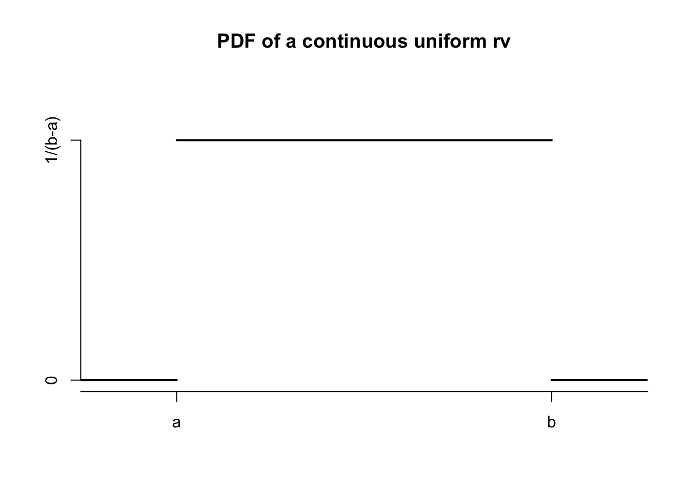
A continuous uniform random variable \(X\) has pdf given by \[ f(x) = \begin{cases} \frac{1}{b -a} & a \le x \le b\\0&{\rm otherwise} \end{cases} \]

A continuous uniform rv \(X\) is characterized by the property that for any interval \(I \subset [a,b]\), the probability \(P(X \in I)\) depends only on the length of \(I\). We write \(X \sim \text{Unif}(a,b)\) if \(X\) is continuous uniform on the interval \([a,b]\).

One example of a random variable that could be modeled by a continous uniform random variable is round-off error in measurements. Say we measure height and record only feet and inches. It is a reasonable first approximation that the error associated with rounding to the nearest inch is uniform on the interval \([-1/2,1/2]\). There may be other sources of measurement error which might not be well modeled by a uniform random variable, but the round-off is uniform.

Another example is related to the Poisson process. If you observe a Poisson process after some length of time \(T\) and see that exactly one event has occurred, then the time that the event occurred in the interval \([0, T]\) is uniformly distributed.

Example 5.58

A random real number is chosen uniformly in the interval 0 to 10. What is the probability that it is bigger than 7, given that it is bigger than 6?

Let \(X \sim \text{Unif}(0,10)\) be the random real number. Then \[ P(X > 7\ |\ X > 6) = \frac{P(X > 7 \cap X > 6)}{P(X > 6)} = \frac{P(X > 7)}{P(X > 6)} =\frac{3/10}{4/10} = \frac{3}{4}. \]

Alternately, we can compute with the punif function, which gives the cdf of a uniform random variable.

(1 - punif(7, 0, 10)) / (1 - punif(6, 0, 10))

## [1] 0.75

The conditional density of a uniform over the interval \([a,b]\) given that it is in the subset \([c,d]\) is uniformly distributed on the interval \([c,d]\). Applying that fact to Example 5.58, we know that \(X\) given \(X > 6\) is uniform on the interval \([6, 10]\). Therefore, the probability that \(X\) is larger than 7 is simply 3/4. Note that this only works for uniform random variables! For other random variables, you need to compute conditional probabilities as in Example 5.58.

We finish this section with a computation of the mean and variance of a uniform random variable \(X\). Not surprisingly, the mean is exactly halfway along the interval of possible values for \(X\).

Theorem 5.17

For \(X \sim \text{Unif}(a,b)\), the expected value of \(X\) is \[ E[X] = \frac{b + a}{2}\] and the variance is \[ \text{var}(X) = \frac{(b - a)^2}{12} \]

Proof:

We compute the mean of \(X\) as follows: \[\begin{align*} E[X]&= \int_a^b \frac{x}{b-a}\, dx\\ &=\frac{x^2}{2(b - a)}|_{x = a}^{x = b}\\ &=\frac{(b - a)(b + a)}{2(b - a)}\\ &=\frac{a+b}{2}. \end{align*}\]

For the variance, first calculate \(E[X^2] = \int_a^b \frac{x^2}{b-a}dx\). Then \[ \text{var}(X) = E[X^2] - E[X]^2 = E[X^2] - \left(\frac{a+b}{2}\right)^2. \] Working the integral and simplifying \(\text{var}(X)\) is left as Exercise 5.26.

3.8.3 Negative binomial

Suppose you repeatedly roll a fair die. What is the probability of getting exactly 14 non-sixes before getting your second 6?

As you can see, this is an example of repeated Bernoulli trials with \(p = 1/6\), but it isn’t exactly geometric because we are waiting for the second success. This is an example of a negative binomial random variable.

Definition 5.59

Suppose that we observe a sequence of Bernoulli trials with probability of success prob. If \(X\) denotes the number of failures x before the nth success, then \(X\) is a negative binomial random variable with parameters n and p. The probability mass function of \(X\) is given by

\[ p(x) = \binom{x + n - 1}{x} p^n (1 - p)^x, \qquad x = 0,1,2\ldots \]

The mean of a negative binomial is \(n p/(1 - p)\), and the variance is \(n p /(1 - p)^2\). The root R function to use with negative binomials is nbinom, so dnbinom is how we can compute values in R. The function dnbinom uses prob for \(p\) and size for \(n\) in our formula.

Example 5.60

Suppose you repeatedly roll a fair die. What is the probability of getting exactly 14 non-sixes before getting your second 6?

dnbinom(x = 14, size = 2, prob = 1 / 6)

## [1] 0.03245274

Note that when size = 1, negative binomial is exactly a geometric random variable, e.g.

dnbinom(x = 14, size = 1, prob = 1 / 6)

## [1] 0.01298109

dgeom(14, prob = 1 / 6)

## [1] 0.01298109

3.8.4 Hypergeometric

Consider the experiment which consists of sampling without replacement from a population that is partitioned into two subgroups - one subgroup is labeled a “success” and one subgroup is labeled a “failure”. The random variable that counts the number of successes in the sample is an example of a hypergeometric random variable.

To make things concrete, we suppose that we have \(m\) successes and \(n\) failures. We take a sample of size \(k\) (without replacement) and we let \(X\) denote the number of successes. Then \[ P(X = x) = \frac{\binom{m}{x} {\binom{n}{k - x}} }{\binom{m + n}{k}} \] We also have \[ E[X] = k (\frac{m}{m + n}) \] which is easy to remember because \(k\) is the number of samples taken, and the probability of a success on any one sample (with no knowledge of the other samples) is \(\frac {m}{m + n}\). The variance is similar to the variance of a binomial as well, \[ V(X) = k \frac{m}{m+n} \frac {n}{m+n} \frac {m + n - k}{m + n - 1} \] but we have the “fudge factor” of \(\frac {m + n - k}{m + n - 1}\), which means the variance of a hypergeometric is less than that of a binomial. In particular, when \(m + n = k\), the variance of \(X\) is 0. Why?

When \(m + n\) is much larger than \(k\), we will approximate a hypergeometric random variable with a binomial random variable with parameters \(n = m + n\) and \(p = \frac {m}{m + n}\). Finally, the R root for hypergeometric computations is hyper. In particular, we have the following example:

Example 5.61

15 US citizens and 20 non-US citizens pass through a security line at an airport. Ten are randomly selected for further screening. What is the probability that 2 or fewer of the selected passengers are US citizens?

In this case, \(m = 15\), \(n = 20\), and \(k = 10\). We are looking for \(P(X \le 2)\), so

sum(dhyper(x = 0:2, m = 15, n = 20, k = 10))

## [1] 0.08677992

3.9 Independent random variables

We say that two random variables, \(X\) and \(Y\), are independent if knowledge of the outcome of \(X\) does not give probabilistic information about the outcome of \(Y\) and vice versa. As an example, let \(X\) be the amount of rain (in inches) recorded at Lambert Airport on a randomly selected day in 2017, and let \(Y\) be the height of a randomly selected person in Botswana. It is difficult to imagine that knowing the value of one of these random variables could give information about the other one, and it is reasonable to assume that the rvs are independent. On the other hand, if \(X\) and \(Y\) are the height and weight of a randomly selected person in Botswana, then knowledge of one variable could well give probabilistic information about the other. For example, if you know a person is 72 inches tall, it is unlikely that they weigh 100 pounds.

We would like to formalize that notion with conditional probability. The natural statement is that for any \(E, F\) subsets of \({\mathbb R}\), the conditional probability \(P(X\in E|Y\in F)\) is equal to \(P(X \in E)\). There are several issues with formalizing the notion of independence that way, so we give a definition that is somewhat further removed from the intuition.

The definition mirrors the multiplication rule for independent events.

Definition 5.62

Suppose \(X\) and \(Y\) are random variables:

\(X\) and \(Y\) are independent \(\iff\) For all \(x\) and \(y\), \(P(X \le x, Y \le y) = P(X \le x) P(Y \le y)\).

For discrete random variables, this is equivalent to saying that \(P(X = x, Y = y) = P(X = x)P(Y = y)\) for all \(x\) and \(y\).

For our purposes, we will often be assuming that random variables are independent.

Example 5.63

Let \(X\) and \(Y\) be uniform random variables on the interval \([0,1]\). Find the cumulative distribution function for the random variable \(Z\) which is the larger of \(X\) and \(Y\).

Let’s start with an observation. Note that \(Z \le z\) exactly when both \(X \le z\) and \(Y \le z\). Therefore, we can rewrite \(F_Z(z) = P(Z \le z) = P(X \le z, Y \le z) = P(X \le z)P(Y \le z)\), where the last equality uses the independence of \(X\) and \(Y\). Since the cdf of a uniform is given by \(F(x) = \begin{cases} 0&x < 0\\x&0\le x \le 1\\1&x > 1\end{cases}\), we obtain the solution of \[ F_Z(z) = \begin{cases}0& z < 0\\z^2&0\le z \le 1\\1&z > 1\end{cases} \]

The pdf of \(Z\) we compute by differentiating \(F_Z(z)\) to get: \[ f_Z(z) = \begin{cases}0& z < 0\\2z&0\le z \le 0\\1&z > 1\end{cases} \]

We can check this by simulation by generating \(X\), \(Y\), and then the maximum of \(X\) and \(Y\). Note that the R function max gives the largest single maximum value of its input. Here, we use pmax which gives the maximum of each pair of elements in the two given vectors.

X <- runif(10000, 0, 1)
Y <- runif(10000, 0, 1)
Z <- pmax(X, Y)
plot(density(Z))

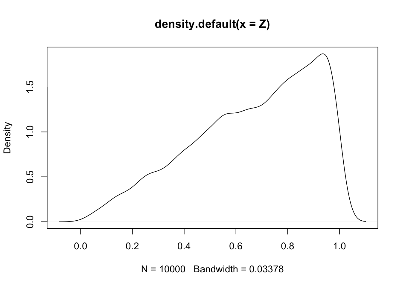
Observe that the distribution of \(Z\) values follows the theoretical pdf function.

Later in this text, we will need to assume that many random variables are independent. We will not make use of the precise mathematical definition later, but for completeness we include it here:

Definition 5.64

We say that the random variables \(X_1, \ldots, X_n\) are independent if for all \(x_1, \ldots, x_n\), \(P(X_1 \le x_1,\ldots, X_n \le x_n) = P(X_1 \le x_1)\cdots P(X_n \le x_n)\).

3.10 Summary

This chapter introduced the notion of a random variable, and the associated notion of a probability distribution. For any random variable, we might be interested in answering probability questions either exactly or through simulation. Usually, these questions involve knowledge of the probability distribution. For some commonly occurring types of random variable, the probability distribution functions are well understood.

Here is a list of the random variables that we introduced in this section, together with pmf/pdf, expected value, variance and root R function.

RV	PMF/PDF	Range	Mean	Variance	R Root
Binomial	\({\binom{n}{x}} p^x(1 - p)^{n - x}\)	\(0\le x \le n\)	\(np\)	\(np(1 - p)\)	binom
Geometric	\(p(1-p)^{x}\)	\(x \ge 0\)	\(\frac{1-p}{p}\)	\(\frac{1-p}{p^2}\)	geom
Poisson	\(\frac {1}{x!} \lambda^x e^{-\lambda}\)	\(x \ge 0\)	\(\lambda\)	\(\lambda\)	pois
Uniform	\(\frac{1}{b - a}\)	\(a \le x \le b\)	\(\frac{a + b}{2}\)	\(\frac{(b - a)^2}{12}\)	unif
Exponential	\(\lambda e^{-\lambda x}\)	\(x \ge 0\)	\(1/\lambda\)	\(1/\lambda^2\)	exp
Normal	\(\frac 1{\sigma\sqrt{2\pi}} e^{(x - \mu)^2/(2\sigma^2)}\)	\(-\infty < x < \infty\)	\(\mu\)	\(\sigma^2\)	norm
Hypergeometric	\(\frac{{\binom{m}{x}} {\binom{n}{k-x}}}{{\binom{m+n}{k}}}\)	\(x = 0,\ldots,k\)	\(kp\)	\(kp(1-p)\frac{m + n - k}{m + n - 1}\)	hyper
Negative Binomial	\(\binom{x + n - 1}{x} p^n (1 - p)^x\)	\(x \ge 0\)	\(n\frac{1-p}p\)	\(n\frac{1-p}{p^2}\)	nbinom

When modeling a count of something, you often need to choose between binomial, geometric, and Poisson. The binomial and geometric random variables both come from Bernoulli trials, where there is a sequence of individual trials each resulting in success or failure. In the Poisson process, events are spread over a time interval, and appear at random.

The normal random variable is a good starting point for continuous measurements that have a central value and become less common away from that mean. Exponential variables show up when waiting for events to occur. Continuous uniform variables sometimes occur as the location of an event in time or space, when the event is known to have happened on some fixed interval.

R provides these random variables (and many more!) through a set of four functions for each known distribution. The four functions are determined by a prefix, which can be p, d, r, or q. The root determines which distribution we are talking about. Each distribution function takes a single argument first, determined by the prefix, and then some number of parameters, determined by the root. The general form of a distribution function in R is:

[prefix][root] ( argument, parameter1, parameter2, ..)

The available prefixes are:

1. p : compute the cumulative distribution function \(P(X < x)\), and the argument is \(x\).
2. d : compute the pdf or pmf \(f\). The value is \(f(x)\), and the argument is \(x\). In the discrete case, this is the probability $P(X = x).
3. r : sample from the rv. The argument is \(N\), the number of samples to take.
4. q : quantile function, the inverse cdf. This computes \(x\) so that \(P(X < x) = q\), and the argument is \(q\).

The distributions we have used in this chapter, with their parameters are:

1. binom is binomial, parameters are \(n\),\(p\).
2. geom is geometric, parameter is \(p\).
3. norm is normal, parameters are \(\mu, \sigma\).
4. pois is Poisson, parameter is \(\lambda\).
5. exp is exponential, parameter is \(\lambda\).
6. unif is uniform, parameters are \(a,b\)

There will be many more distributions to come, and the four prefixes work the same way for all of them.

Vignette: An R Markdown Primer

RStudio has included a method for making higher quality documents from a combination of R code and some basic markdown formatting, which is called R Markdown. For students reading this book, writing your homework in RMarkdown will allow you to have reproducible results. It is much more efficient than creating plots in R and copy/pasting into Word or some other document. Professionals may want to write reports in RMarkdown. This chapter gives the basics, with a leaning toward homework assignments.

In order to create an R Markdown file, inside RStudio you click on File, then New File and R Markdown. You will be prompted to enter a Title and an Author. For now, leave the Default Output Format as .html and leave the Document icon highlighted. When you have entered an acceptable title and author, click OK and a new tab in the Source pane should open up. (That is the top left pane in RStudio.) The very first thing that we would do is click on the Knit button right above the source panel. It should knit the document and give you a nice-ish looking document. Our goal in this vignette is to get you started making nicer looking homework and other documents in RMarkdown. For further information, see Xie, Allaire and Grolemund’s book¹²

You should see something that looks like this, with some more things underneath.

---
title: “Untitled”
author: “Darrin Speegle”
date: “1/20/2021”
output: html_document
---

This part of the code is the YAML (YAML Ain’t Markup Language). Next is a bit of code that starts like this. You don’t have to change that, but you might experiment with the tufte style. You will need to install the tufte package in order to do this, and change your YAML to look like this.

---
title: "Homework 1"
author: "Darrin Speegle"
date: "1/20/2021"
output:
  tufte::tufte_handout: default
  tufte::tufte_html: default
---

```{r setup, include=FALSE}
knitr::opts_chunk$set(echo = TRUE, 
                      message = FALSE, 
                      warning = FALSE, 
                      fig.width = 4, 
                      fig.height = 4, 
                      fig.margin = TRUE)
```

One benefit of using the tufte package is that in order for the document to look good, it requires you to write more text than you might otherwise. Many beginners tend to have too much R code and output (including plots), and not enough words. If you use the tufte package, you will see that the document doesn’t look right unless the proportion of words to plots and other elements is better.

Note that we have changed the title of the homework, and the default values for several things in the file. That is, we changed knitr::opts_chunk$set(echo = TRUE) to read knitr::opts_chunk$set(echo = TRUE, message = FALSE, warning = FALSE, fid.width = 4, fig.height = 4, fig.margin = TRUE). You should experiment with these options to find the set-up that works best for you. If you are preparing a document for presentation, for example, you would most likely want to have echo = FALSE.

Once you have made those changes to your own file, click on the Knit button just above the Source pane. A window should pup up that says Homework 1, followed by your name and the date that you entered. If that didn’t happen, redo the above. Note that the figures appear in the margins of the text. Often, this is what we want, because otherwise the figures don’t line up well with where we are reading. However, if there is a large figure, then this will not work well. You would then add fig.fullwidth = TRUE as an option to your chunk like this.

``` {r fig.fullwidth = TRUE}

For the purposes of this primer, we are mostly assuming that you are typing up solutions to a homework. Add the following below the file you have already created and Knit again.

1. Consider the `DrinksWages` data set in the `HistData` package.
a. Which trade had the lowest wages?

```{r}
DrinksWages[which.min(DrinksWages$wage),]
```

We see that **factory worker** had the lowest wages; 12 shillings per week. 
If there had been multiple professions with a weekly wage of 12 shillings per week, 
then we would have only found one of them here.

b. Provide a histogram of the wages of the trades

```{r}
hist(DrinksWages$wage)
```

The weekly wages of trades in 1910 was remarkably symmetric. Values ranged from a 
low of 12 shillings per week for factory workers to a high of 40 shillings per 
week for rivetters and glassmakers. 

Notes

1. putting a 1. at the beginning of a line will start a numbered list.
2. Putting mtcars in single quotes will make the background shaded, so that it is clear that it is an R object of some sort. Putting ** before and after a word or phrase makes it bold.
3. The part beginning with ```{r} and ending with ``` is called an R chunk. You can create a new R chunk by using Command + Alt + I. When you knit your file, R Markdown puts the commands that it used in a shaded box, to indicate that it is R code. Then, it also executes the R commands and shows the output.
4. Text should not be inside of the R chunk. You should put your text either above or below the chunk.
5. Every R chunk probably needs to have some sort of explanation in words. Just giving the R code is often not sufficient for someone to understand what you are doing. You will need to explain what it is you have done. (This can often be done quite quickly, but sometimes can take quite a bit of time.)
6. If you are using a package inside R Markdown, you must load the package inside your markdown file! We recommend loading all libraries at the top of the markdown file.
7. You can include math via LaTeX commands. LaTeX is a very powerful word processor that produces high quality mathematical formulas. A couple of useful examples are $x^2$, which is \(x^2\), or $X_i$, which is \(X_i\).
8. You can knit to .html, .pdf or .doc format. We like .pdf the best, but it requires that TeX be installed on your computer. If you don’t have it installed, then you will need to use the following to R commands to install it.

install.packages('tinytex')
tinytex::install_tinytex()  

In order to finish typing up the solutions to Homework 1, you would continue with your list of problems, and insert R chunks with the R code that you need plus some explanation in words for each problem.

When you are done, you should Knit the document again, and a new .html or .pdf will appear. The last thing we would say is that Markdown has a lot more typesetting that it can do than what we have indicated up to this point. There are many more good resources on this, for example Grolemund and Wickham, Ismay, or you can look at the tufte template in RStudio by clicking on File -> New File -> R Markdown -> From Template -> Tufte Handout.

Exercises

5.1

Let \(X\) be a discrete random variable with probability mass function given by \[ p(x) = \begin{cases} 1/4 & x = 0 \\ 1/2 & x = 1\\ 1/8 & x = 2\\ 1/8 & x = 3 \end{cases} \]

1. Verify that \(p\) is a valid probability mass function.
2. Find the mean of \(X\).
3. Find \(P(X \ge 2)\).
4. Find \(P(X \ge 2\ |\ X \ge 1)\).

5.2

Find the variance and standard deviation of the rv \(X\) from Exercise 5.1.

5.3

Roll two ordinary dice and let \(X\) be their sum. Compute the pmf for X. Compute the mean and standard deviation of \(X\).

5.4

Suppose you roll two ordinary dice. Calculate the expected value of their product.

5.5

Suppose that a hat contains slips of papers containing the numbers 1, 2 and 3. Two slips of paper are drawn without replacement. Calculate the expected value of the product of the numbers on the slips of paper.

5.6

Pick an integer from 0 to 999 with all possible numbers equally likely. What is the expected number of digits in your number?

5.7

To play the Missouri lottery Pick 3, you choose three digits 0-9 in order. Later, the lottery selects three digits at random, and you win if your choices match the lottery values in some way. Here are some possible bets you can play:

1. $1 Straight wins if you correctly guess all three digits, in order. It pays $600.
2. $1 Front Pair wins if you correctly guess the first two digits. It pays $60.
3. $1 Back Pair wins if you correctly guess the last two digits. It pays $60.
4. $6 6-way combo wins if the three digits are different and you guess all three in any order. It pays $600.
5. $3 3-way combo wins if two of the three digits are the same, and you guess all three in any order. It pays $600.
6. $1 1-off wins if you guess all three digits in the correct order, but one of your guesses is off by one (so instead of 7 you guessed 6 or 8). 9 and 0 are considered one-off. It pays $29.

Consider the value of your bet to be your expected winnings per dollar bet. What value do each of these bets have?

5.8

Suppose you take a 20 question multiple choice test, where each question has four choices. You guess randomly on each question. What is your expected score? What is the probability you get 10 or more questions correct?

5.9

Steph Curry is a 91% free throw shooter. If he shoots 10 free throws in a game, what is his expected number of shots made? What is the probability that he makes at least 8 free throws?

5.10

Suppose 27 people write their names down on slips of paper and put them in a hat. Each person then draws one name from the hat. Estimate the expected value and standard deviation of the number of people who draw their own name. (Assume no two people have the same name!)

5.11

Suppose that 55% of voters support Proposition A.

1. You poll 200 voters. What is the expected number that support the measure?
2. What is the margin of error for your poll (two standard deviations)?
3. What is the probability that your poll claims that Proposition A will fail?
4. How large a poll would you need to reduce your margin of error to 2%?

5.12

Plot the pdf and cdf of a uniform random variable on the interval \([0,1]\).

5.13

Compare the cdf and pdf of an exponential random variable with rate \(\lambda = 2\) with the cdf and pdf of an exponential rv with rate 1/2. (If you wish to read ahead in Chapter 4, you can learn how to put plots on the same axes, with different colors.)

5.14

Compare the pdfs of three normal random variables, one with mean 1 and standard deviation 1, one with mean 1 and standard deviation 10, and one with mean -4 and standard deviation 1.

5.15

Let \(X\) be a random variable with pdf \(f(x) = 3(1 - x)^2\) when \(0\le x \le 1\), and \(f(x) = 0\) otherwise.

1. Verify that \(f\) is a valid pdf.
2. Find the mean and variance of \(X\).
3. Find \(P(X \ge 1/2)\).
4. Find \(P(X \ge 1/2\ |\ X \ge 1/4)\).

5.16

Let \(X\) be a normal rv with mean 1 and standard deviation 2.

1. Find \(P(a \le X \le a + 2)\) when \(a = 3\).
2. Sketch the graph of the pdf of \(X\), and indicate the region that corresponds to your answer in the previous part.
3. Find the value of \(a\) such that \(P(a \le X \le a + 2)\) is the largest.

5.17

Let \(X\) be an exponential rv with rate \(\lambda = 1/4\).

1. What is the mean of \(X\)?
2. Find the value of \(a\) such that \(P(a \le X \le a + 1)\) is maximized. Is the mean contained in the interval \([a, a+1]\)?

5.18

For each of the following functions, decide whether the function is a valid pdf, a valid cdf or neither.

1. \(h(x) = \begin{cases} 1&0\le x \le 2\\-1&2\le x\le 3\\0&{\rm {otherwise}} \end{cases}\)
2. \(h(x) = \sin(x) + 1\)
3. \(h(x) = \begin{cases} 1 - e^{-x^2}& x\ge 0\\0& x< 0\end{cases}\)
4. \(h(x) = \begin{cases} 2xe^{-x^2}&x\ge 0\\0&x < 0\end{cases}\)

5.19

Provide an example of a pdf \(f\) for a random variable \(X\) such that there exists an \(x\) for which \(f(x) > 1\). Is it possible to have \(f(x) > 1\) for all values of \(x\)?

5.20

Is there a function which is both a valid pdf and a valid cdf? If so, give an example. If not, explain why not.

5.21

Let \(X\) be a random variable with mean \(\mu\) and standard deviation \(\sigma\). Find the mean and standard deviation of \(\frac{X - \mu}{\sigma}\).

5.22

Let \(X_1, X_2, X_3\) be independent uniform random variables on the interval \([0,1]\). Find the cdf of the random variable \(Z\) which is the maximum of \(X_1, X_2\) and \(X_3\).

5.23

Suppose the time (in seconds) it takes your professor to set up their computer to start class is uniformly distributed on the interval \([0, 30]\). Suppose also that it takes you 5 seconds to send your mom a nice, quick text that you are thinking of her. You only text her if you can complete it during the time your professor is setting up their computer. If you try to text your mom every day in class, what is the probability that she will get a text on 3 consecutive days?

5.24

In the summer of 2020, the U.S. was considering pooled testing of COVID-19<sup>13</sup>. This problem explores the math behind pooled testing. Since the availability of tests is limited, the testing center proposes the following pooled testing technique:

• Two samples are randomly selected and combined. The combined sample is tested.
• If the combined sample tests negative, then both people are assumed negative.
• If the combined sample tests positive, then both people need to be retested for the disease.

Suppose in a certain population, 5 percent of the people being tested for COVID-19 actually have COVID-19. Let \(X\) be the total number of tests that are run.

1. What is the pmf of \(X\)?
2. What is the expected value of \(X\)?
3. Repeat the above, but imagine that three samples are combined. If it is positive, then all three people need to be retested.
4. If your only concern is to minimize the expected number of tests given to the population, which technique would you recommend?

5.25

Suppose the time to failure (in years) for a particular component is distributed as an exponential random variable with rate \(\lambda = 1/5\). For better performance, the system has two components installed, and the system will work as long as either component is functional. Assume the time to failure for the two components is independent. What is the probability that the system will fail before 10 years has passed?

5.26

Verify that a uniform random variable on the interval \([a,b]\) has variance given by \(\sigma^2 = \frac{(b - a)^2}{12}\).

5.27 (memoryless property)

Let \(X\) be an exponential random variable with rate \(\lambda\). If \(a\) and \(b\) are positive numbers, then \[ P(X > a + b\ |\ X > b) = P(X > a) \]

1. Explain why this is called the memoryless property.
2. Show that for an exponential rv \(X\) with rate \(\lambda\), \(P(X > a) = e^{-a\lambda}\).
3. Use the result in (b) to prove the memoryless property for exponential random variables.

5.28

Suppose that scores on an exam are normally distributed with mean 80 and standard deviation 5.

1. What is the probability that a student scores higher than 85 percent on the exam?
2. Assume that exam scores are independent and that 10 students take the exam. What is the probability that 4 or more students score 85 percent or higher on the exam?

5.29

Let \(X\) be a Poisson rv with mean 3.9.

1. Create a plot of the pmf of \(X\).
2. What is the most likely outcome of \(X\)?
3. Find \(a\) such that \(P(a \le X \le a + 1)\) is maximized.
4. Find \(b\) such that \(P(b \le X \le b + 2)\) is maximized.

5.30

Let \(X\) be a random variable whose pdf is given by the plot below. Assume that the pdf is zero outside of the interval given in the plot.

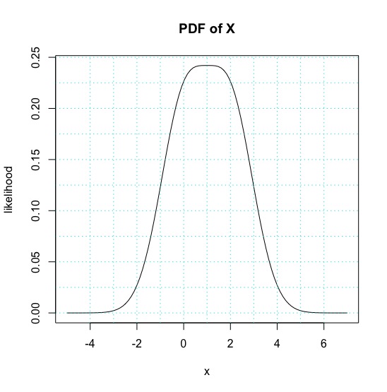
1. Estimate the mean of \(X\).
2. Estimate the standard deviation of \(X\).
3. For which \(a\) is \(P(a \le X \le a + 2)\) maximized?
4. Estimate \(P(0 \le X \le 2)\).

5.31

We stated in the text that a Poisson random variable \(X\) with rate \(\lambda\) is approximately a Binomial random variable \(Y\) with \(n\) trials and probability of success \(\lambda/n\) when \(n\) is large. Suppose \(\lambda = 2\) and \(n = 300\). What is the largest absolute value of the difference between \(P(X = x)\) and \(P(Y = x)\)?

5.32

For each of the following descriptions of a random variable, indicate whether it can best be modeled by binomial, geometric, Poisson, uniform, exponential or normal. Answer the associated questions. Note that not all of the experiments yield rv’s that are exactly of the type listed above, but we are asking about reasonable modeling.

1. Let \(Y\) be the random variable that counts the number of sixes which occur when a die is tossed 10 times. What type of random variable is \(Y\)? What is \(P(Y=3)\)? What is the expected number of sixes? What is \({\rm Var}(Y)\)?
2. Let \(U\) be the random variable which counts the number of accidents which occur at an intersection in one week. What type of random variable is \(U\)? Suppose that, on average, 2 accidents occur per week. Find \(P(U=2)\), \(E(U)\) and \({\rm Var}(U)\).
3. Suppose a stop light has a red light that lasts for 60 seconds, a green light that lasts for 30 seconds and a yellow light that lasts for 5 seconds. When you first observe the stop light, it is red. Let \(X\) denote the time until the light turns green. What type of rv would be used to model \(X\)? What is its mean?
4. Customers arrive at a teller’s window at a uniform rate of 5 per hour. Let \(X\) be the length in minutes of time that the teller has to wait until they see their first customer after starting their shift. What type of rv is \(X\)? What is its mean? Find the probability that the teller waits less than 10 minutes for their first customer.
5. A coin is tossed until a head is observed. Let \(X\) denote the total number of tails observed during the experiment. What type of rv is \(X\)? What is its mean? Find \(P(X \le 3)\).
6. Let \(X\) be the recorded body temperature of a healthy adult in degrees Fahrenheit. What type of rv is \(X\)? Estimate its mean and standard deviation, based on your knowledge of body temperatures.

5.33

Suppose you turn on a soccer game and see that the score is 1-0 after 30 minutes of play. Let \(X\) denote the time (in minutes from the start of the game) that the goal was scored. What type of rv is \(X\)? What is its mean?

5.34

The charge \(e\) on one electron is too small to measure. However, one can make measurements of the current \(I\) passing through a detector. If \(N\) is the number of electrons passing through the detector in one second, then \(I = eN\). Assume \(N\) is Poisson. Show that the charge on one electron is given by \(\frac{{\rm var}(I)}{E[I]}\).

5.35

Climbing rope will break if pulled hard enough. Experiments show that 10.5mm Dynamic nylon rope has a mean breaking point of 5036 lbs with a standard deviation of 122 lbs. Assume breaking points of rope are normally distributed.

1. Sketch the distribution of breaking points for this rope.
2. What proportion of ropes will break with 5000 lbs of load?
3. At what load will 95% of all ropes break?

5.36

There exist naturally occurring random variables that are neither discrete nor continuous. Suppose a group of people is waiting for one more person to arrive before starting a meeting. Suppose that the arrival time of the person is exponential with mean 4 minutes, and that the meeting will start either when the person arrives, or after 5 minutes, whichever comes first. Let \(X\) denote the length of time the group waits before starting the meeting.

1. Find \(P(0 \le X \le 4)\).
2. Find \(P(X = 5)\).

5.37

In this exercise, we verify Theorem 5.10 in a special case. Let \(X\) be normal with mean 0 and standard deviation 2, and let \(Y\) be normal with mean 0 and standard deviation 1. Assume \(X\) and \(Y\) are independent. Use simulation to estimate the variance of \(X + 3Y\), and compare to \(1^2 \times 4 + 3^2 \times 1\).

5.38

A roulette wheel has 38 slots and a ball that rolls until it falls into one of the slots, all of which are equally likely. Eighteen slots are black numbers, eighteen are red numbers, and two are green zeros. If you bet on “red”, and the ball lands in a red slot, the casino pays you your bet, otherwise the casino wins your bet.

1. What is the expected value of a $1 bet on red?
2. Suppose you bet $1 on red, and if you win you “let it ride” and bet $2 on red. What is the expected value of this plan?

5.39

One (questionable) roulette strategy is called bet doubling: You bet $1 on red, and if you win, you pocket the $1. If you lose, you double your bet so you are now betting $2 on red, but have lost $1. If you win, you win $2 for a $1 profit, which you pocket. If you lose again, you double your bet to $4 (having already lost $3). Again, if you win, you have $1 profit, and if you lose, you double your bet again. This guarantees you will win $1, unless you run out of money to keep doubling your bet.

1. Say you start with a bankroll of $127. How many bets can you lose in a row without losing your bankroll?
2. If you have a $127 bankroll, what is the probability that bet doubling wins you $1?
3. What is the expected value of the bet doubling strategy with a $127 bankroll?
4. If you play the bet doubling strategy with a $127 bankroll, how many times can you expect to play before you lose your bankroll?

5.40

Flip a fair coin 10 times and let \(X\) be the proportion of times that a Head is followed by another Head. Discard the sequence of ten tosses if you don’t obtain a Head in the first 9 tosses. What is the expected value of \(X\)? (Note: this is not asking you to estimate the conditional probability of getting Heads given that you just obtained Heads.)

See Miller and Sanjurjo<sup>14</sup> for a connection to the “hot hand” fallacy.

1.1

In an experiment<sup>15</sup> to test whether participants have absolute pitch, scientists play notes and the participants say which of the 12 notes is being played. The participant gets one point for each note that is correctly identified, and 3/4 of a point for each note that is off by a half-step. (Note that if the possible guesses are 1:12, then the difference between 1 and 12 is a half-step, as is the difference between any two values that are one apart.)

1. If the participant hears 36 notes and randomly guesses each time, what is the expected score of the participant?
2. If the participant hears 36 notes and randomly guesses each time, what is the standard deviation of the score of the participant?

??.1

Let \(X \sim \text{Geom}(p)\) be a geometric rv with success probability \(p\). Show that the standard deviation of \(X\) is \(\frac{\sqrt{1-p}}{p}\). Hint: Follow the proof of Theorem 5.6 but take the derivative twice with respect to \(q\). This will compute \(E[X(X-1)]\). Use \(E[X(X-1)] = E[X^2] - E[X]\) and Theorem 5.9 to finish.

??.2

This problem was reported to be a Google interview question. Suppose you have a stick of length one meter. You randomly select two points on the stick, and break the stick at those two places. Estimate the probability that the resulting three pieces of stick can be used to form a triangle.

??.3

The Gaussian Integral. There is no elementary antiderivative for the function \(e^{x^2}\). However, the Gaussian integral \(\int_{-\infty}^\infty e^{-x^2} dx\) can be computed exactly. Begin with the following: \[ \left(\int_{-\infty}^\infty e^{-x^2} dx\right)^2 = \int_{-\infty}^{\infty} e^{-x^2}\,dx \int_{-\infty}^{\infty} e^{-y^2}\,dy = \int_{-\infty}^{\infty} \int_{-\infty}^{\infty} e^{-(x^2+y^2)}\, dx\,dy \] Now switch to polar coordinates and show that the Gaussian integral is equal to \(\sqrt{\pi}\)

??.4

As stated in the text, the pdf of a Poisson random variable \(X \sim \text{Pois}(\lambda)\) is \[ p(x) = \frac 1{x!} \lambda^x e^{-\lambda}, \quad x = 0,1,\ldots \]

Prove the following:

1. \(p\) is a pdf. (You need to show that \(\sum_{x=0}^{\infty} p(x) = 1\).)
2. \(E(X) = \lambda.\)
3. \(\text{var}(X) = \lambda.\)

Simulation of Random Variables

In this chapter we discuss simulation related to random variables. We will simulate probabilities related to random variables, and more importantly for our purposes, we will simulate pdfs and pmfs of random variables.

Estimating probabilities of rvs via simulation

In order to run simulations with random variables, we will use the R command r + distname, where distname is the name of the distribution, such as unif, geom, pois, norm, exp or binom. The first argument to any of these functions is the number of samples to create.

Most distname choices can take additional arguments that affect their behavior. For example, if I want to create a random sample of size 100 from a normal random variable with mean 5 and sd 2, I would use rnorm(100, mean = 5, sd = 2), or simply rnorm(100, 5, 2). Without the additional arguments, rnorm gives the standard normal random variable, with mean 0 and sd 1. For example, rnorm(10000) gives 10000 random values of the standard normal random variable \(Z\).

Our strategy for estimating probabilities using simulation is as follows. We first create a large (approximately 10,000) sample from the distribution(s) in question. Then, we use the mean function to compute the percentage of times that the event we are interested in occurs. If the sample size is reasonably large and representative, then the true probability that the event occurs should be close to the percentage of times that the event occurs in our sample. It can be useful to repeat this procedure a few times to see what kind of variation we obtain in our answers.

Example 1.1

Let \(Z\) be a standard normal random variable. Estimate \(P(Z > 1)\).

We begin by creating a large random sample from a normal random variable.

simdata <- rnorm(10000)

Next, we compute the percentage of times that the sample is greater than one. First, we create a vector that contains TRUE at each index of the sample that is greater than one, and contains FALSE at each index of the sample that is less than or equal to one.

log_vec <- simdata > 1
head(log_vec)

## [1] FALSE FALSE FALSE FALSE  TRUE FALSE

Now, we count the number of times we see a TRUE, and divide by the length of the vector.

sum(log_vec == TRUE)/10000

## [1] 0.1664

There are a few improvements we can make. First, log_vec == TRUE is just the same as log_vec, so we can compute

sum(log_vec)/10000

## [1] 0.1664

Lastly, we note that sum converts TRUE to 1 and FALSE to zero. We are adding up these values and dividing by the length, which is the same thing as taking the mean. So, we can just do

mean(log_vec)

## [1] 0.1664

For simple problems, it is often easier to omit the intermediate step(s) and write

mean(simdata > 1)

## [1] 0.1664

Example 1.2

Let \(Z\) be a standard normal rv. Estimate \(P(Z^2 > 1)\).

simdata <- rnorm(10000)
mean(simdata^2 > 1)

## [1] 0.3232

We can also easily estimate means and standard deviations of random variables. To do so, we create a large random sample from the distribution in question, and we take the sample mean or sample standard deviation of the large sample. If the sample is large and representative, then we expect the sample mean to be close to the true mean, and the sample standard deviation to be close to the true standard deviation. Let’s begin with an example where we know what the correct answer is, in order to check that the technique is working.

Example 1.3

Let \(Z\) be a normal random variable with mean 0 and standard deviation 1. Estimate the mean and standard deviation of \(Z\).

simdata <- rnorm(10000, 0, 1)
mean(simdata)

## [1] 0.002707796

sd(simdata)

## [1] 0.9868997

We see that we are reasonably close to the correct answers of 0 and 1.

Example 1.4

Estimate the mean and standard deviation of \(Z^2\).

simdata <- rnorm(10000)
mean(simdata^2)

## [1] 0.9981349

sd(simdata^2)

## [1] 1.410338

We will see later in this chapter that \(Z^2\) is a \(\chi^2\) random variable with one degree of freedom, and it is known that a \(\chi^2\) random variable with \(\nu\) degrees of freedom has mean \(\mu\) and standard deviation \(\sqrt{2\nu}\). Thus, the answers above are pretty close to the correct answers.

Example 1.5

Let \(X\) and \(Y\) be independent standard normal random variables. Estimate \(P(XY > 1)\).

There are two ways to do this. The first is:

x <- rnorm(10000)
y <- rnorm(10000)
mean(x*y > 1)

## [1] 0.1013

A technique that is closer to what we will be doing below is the following. We want to create a random sample from the random variable \(Z = XY\). To do so, we would use

simdata <- rnorm(10000) * rnorm(10000)

Note that R multiples the vectors componentwise. Then, we compute the percentage of times that the sample is greater than 1 as before.

mean(simdata > 1)

## [1] 0.1038

The two methods give different but similar answers because simulations are random and only estimate the true values.

Note that \(P(XY > 1)\) is not the same as the answer we got for \(P(Z^2 > 1)\) in Example 1.4.

Estimating discrete distributions

In this section, we show how to estimate via simulation the pmf of a discrete random variable. Let’s begin with an example.

Example 1.6

Suppose that two dice are rolled, and their sum is denoted as \(X\). Estimate the pmf of \(X\) via simulation.

To estimate \(P(X = 2)\), for example, we would use

simdata <- replicate(10000, {
  dieRoll <- sample(1:6, 2, TRUE)
  sum(dieRoll)
})
mean(simdata == 2)

## [1] 0.0289

It is possible to repeat this replication for each value \(2,\ldots, 12\), but that would take a long time. More efficient is to keep track of all of the observations of the random variable, and divide each by the number of times the rv was observed. We will use table for this. Recall, table gives a vector of counts of each unique element in a vector. That is,

table(c(1,1,1,1,1,2,2,3,5,1))

## 
## 1 2 3 5 
## 6 2 1 1

indicates that there are 6 occurrences of “1”, 2 occurrences of “2”, and 1 occurrence each of “3” and “5”. To apply this to the die rolling, we create a vector of length 10,000 that has all of the observances of the rv \(X\), in the following way:

simdata <- replicate(10000, {
  dieRoll <- sample(1:6, 2, TRUE)
  sum(dieRoll)
})
table(simdata)

## simdata
##    2    3    4    5    6    7    8    9   10   11   12 
##  300  547  822 1080 1412 1655 1418 1082  846  562  276

We then divide each entry of the table by 10,000 to get the estimate of the pmf:

table(simdata)/10000

## simdata
##      2      3      4      5      6      7      8      9     10     11 
## 0.0300 0.0547 0.0822 0.1080 0.1412 0.1655 0.1418 0.1082 0.0846 0.0562 
##     12 
## 0.0276

We don’t want to hard-code the 10000 value in the above command, because it can be a source of error if we change the number of replications and forget to change the denominator here. There is a base R function proportions <sup>16</sup> which is useful for dealing with tabled data. In particular, if the tabled data is of the form above, then it computes the proportion of each value.

proportions(table(simdata))

## simdata
##      2      3      4      5      6      7      8      9     10     11 
## 0.0300 0.0547 0.0822 0.1080 0.1412 0.1655 0.1418 0.1082 0.0846 0.0562 
##     12 
## 0.0276

And, there is our estimate of the pmf of \(X\). For example, we estimate the probability of rolling an 11 to be 0.0562.

The function proportions is discussed further in Section 7.1.

Example 1.7

Suppose fifty randomly chosen people are in a room. Let \(X\) denote the number of people in the room who have the same birthday as someone else in the room. Estimate the pmf of \(X\).

Tryit ??.2

Before reading further, what do you think the most likely outcome of \(X\) is?

We will simulate birthdays by taking a random sample from 1:365 and storing it in a vector. The tricky part is counting the number of elements in the vector that are repeated somewhere else in the vector. We will create a table and add up all of the values that are bigger than 1. Like this:

birthdays <- sample(1:365, 50, replace = TRUE)
table(birthdays)

## birthdays
##   8   9  13  20  24  41  52  64  66  70  92  98  99 102 104 119 123 126 
##   2   1   1   2   2   1   1   1   1   1   1   1   1   1   1   1   1   1 
## 151 175 179 182 185 222 231 237 240 241 249 258 259 276 279 285 287 313 
##   1   1   1   1   1   1   1   1   1   1   1   1   2   2   1   1   1   1 
## 317 323 324 327 333 344 346 364 365 
##   1   1   1   1   1   1   1   1   1

We look through the table and see that anywhere there is a number bigger than 1, there are that many people who share that birthday. To count the number of people who share a birthday with someone else:

sum(table(birthdays)[table(birthdays) > 1])

## [1] 10

Now, we put that inside replicate, just like in the previous example.

## simdata
##      0      2      3      4      5      6      7      8      9     10 
## 0.0309 0.1196 0.0059 0.1982 0.0219 0.2146 0.0309 0.1688 0.0293 0.0917 
##     11     12     13     14     15     16     17     18     19     21 
## 0.0205 0.0361 0.0097 0.0137 0.0034 0.0034 0.0006 0.0006 0.0001 0.0001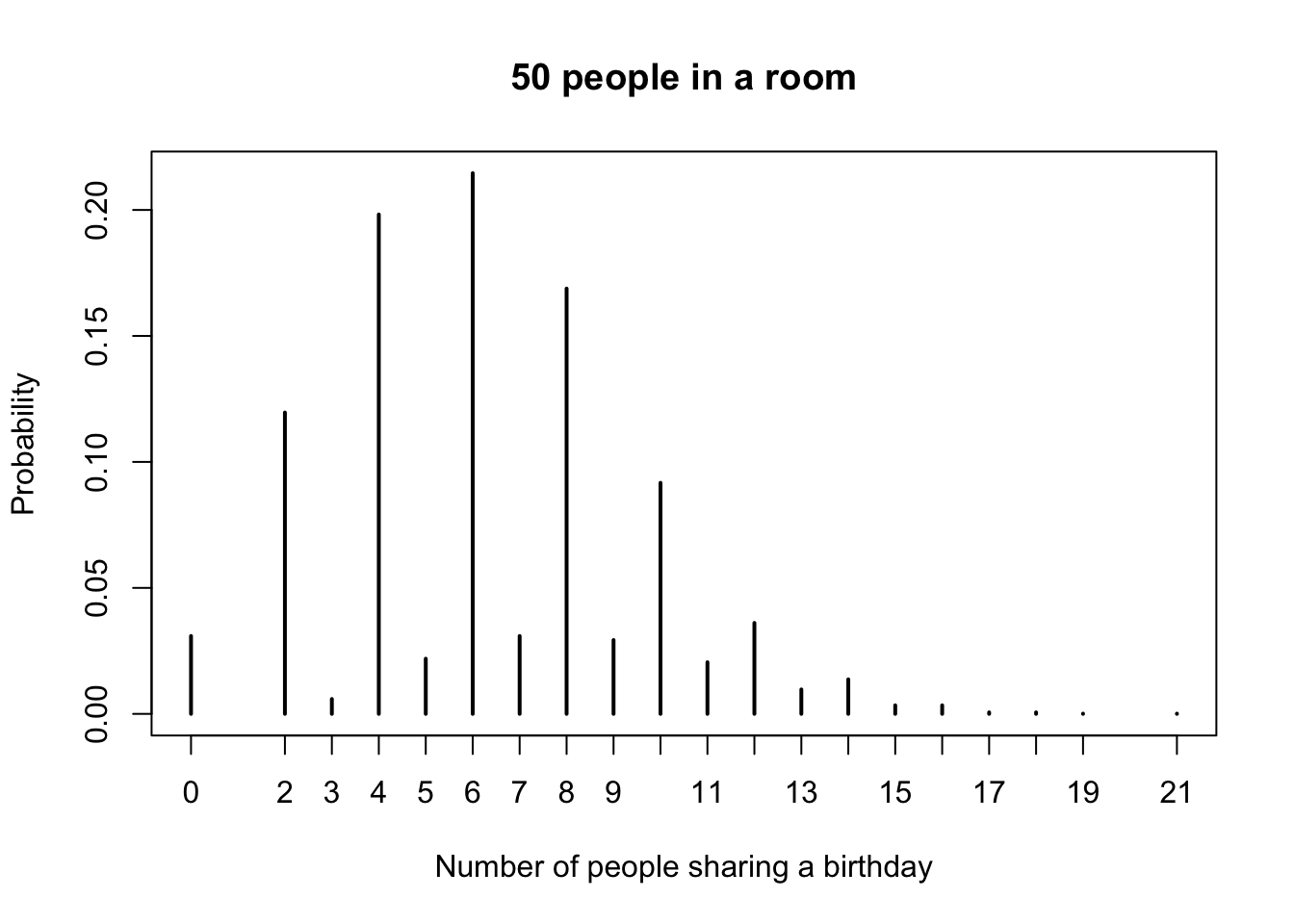

simdata <- replicate(10000, {
  birthdays <- sample(1:365, 50, replace = TRUE)
  sum(table(birthdays)[table(birthdays) > 1])
})
pmf <- proportions(table(simdata))
pmf
plot(pmf, main="50 people in a room",
     xlab = "Number of people sharing a birthday",
     ylab = "Probability")

Looking at the pmf, our best estimate is that the most likely outcome is that 6 people in the room share a birthday with someone else, followed closely by 4 and then 8. Note that it is impossible for exactly one person to share a birthday with someone else in the room! It would be preferable for several reasons to have the observation \(P(X = 1) = 0\) listed in the table above, but we leave that for another day.

Example 1.8

You toss a coin 100 times. After each toss, either there have been more heads, more tails, or the same number of heads and tails. Let \(X\) be the number of times in the 100 tosses that there were more heads than tails. Estimate the pmf of \(X\).

Tryit ??.3

Before looking at the solution, guess whether the pmf of \(X\) will be centered around 50, or not.

We start by doing a single run of the experiment. Recall that the function cumsum accepts a numeric vector and returns the cumulative sum of the vector. So, cumsum(c(1, 3, -1)) would return c(1, 4, 3).

coin_flips <- sample(c("H", "T"), 100, replace = TRUE) #flip 100 coins
num_heads <- cumsum(coin_flips == "H") #cumulative number of heads so far
num_tails <- cumsum(coin_flips == "T") #cumulative number of tails so far
sum(num_heads > num_tails) #number of times there were more heads than tails

## [1] 0

Now, we put that inside of replicate.

simdata <- replicate(100000, {
  coin_flips <- sample(c("H", "T"), 100, replace = TRUE)
  num_heads <- cumsum(coin_flips == "H")
  num_tails <- cumsum(coin_flips == "T")
  sum(num_heads > num_tails) 
})
pmf <- proportions(table(simdata))

When we have this many possible outcomes, it is easier to view a plot of the pmf than to look directly at the table of probabilities.

plot(pmf, ylab = "Probability", xlab = "More heads than tails")

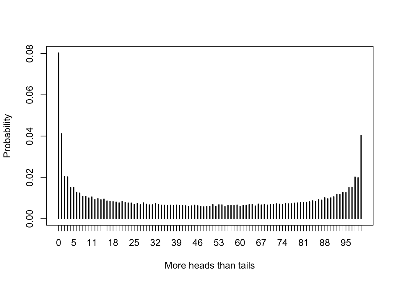
The most likely outcome (by far) is that there are never more heads than tails in the 100 tosses of the coin. This result can be surprising, even to experienced mathematicians.

Example 1.9

Suppose you have a bag full of marbles; 50 are red and 50 are blue. You are standing on a number line, and you draw a marble out of the bag. If you get red, you go left one unit. If you get blue, you go right one unit. This is called a random walk. You draw marbles up to 100 times, each time moving left or right one unit. Let \(X\) be the number of marbles drawn from the bag until you return to 0 for the first time. The rv \(X\) is called the first return time since it is the number of steps it takes to return to your starting position.

Estimate the pmf of \(X\).

movements <- sample(rep(c(1, -1), times = 50), 100, FALSE)
movements[1:10]

##  [1] -1  1  1 -1  1 -1  1 -1  1  1

cumsum(movements)[1:10]

##  [1] -1  0  1  0  1  0  1  0  1  2

which(cumsum(movements) == 0)

##  [1]   2   4   6   8  22  28  30  32  34  36  86  94  96  98 100

min(which(cumsum(movements) == 0))

## [1] 2

Now, we just need to table it like we did before.

simdata <- replicate(10000, {
  movements <- sample(rep(c(1, -1), times = 50), 100, FALSE)
  min(which(cumsum(movements) == 0)) 
})
pmf <- proportions(table(simdata))
plot(pmf, main="First return time for a 100 step random walk",
     xlab = "Steps to return",
     ylab = "Probability")

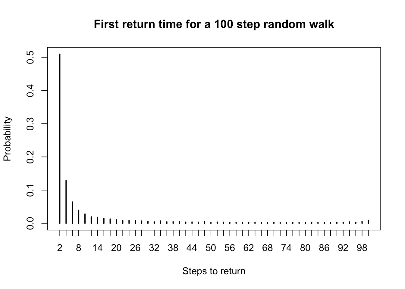
Estimating continuous distributions

In this section, we show how to estimate the pdf of a continuous rv via simulation. As opposed to the discrete case, we will not get explicit values for the pdf, but we will rather get a graph of it. ˜ ::: {.example #exm:twoZ}

Estimate the pdf of \(2Z\) when \(Z\) is a standard normal random variable

Our strategy is to take a random sample of size 10,000 and use either the density or the hist function to estimate the pdf. As before, we build our sample of size 10,000 up as follows:

A single value sampled from standard normal rv:

z <- rnorm(1)

We multiply it by 2 to get a single value sampled from \(2Z\).

2 * z

## [1] 0.03234922

Now create 10,000 values of \(2Z\):

zData <- 2 * rnorm(10000)

We then use density to estimate and plot the pdf of the data:

plot(density(zData),
     main = "Density of 2Z",
     xlab = "2Z")

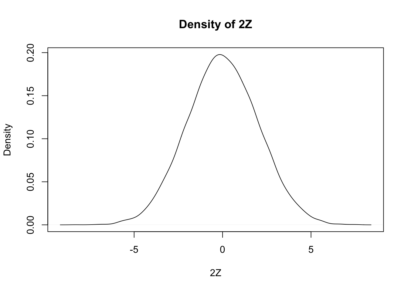
Notice that the most likely outcome of \(2Z\) seems to be centered around 0, just as it is for \(Z\), but that the spread of the distribution of \(2Z\) is twice as wide as the spread of \(Z\).

Alternatively, we could have created a histogram of the data, using hist. We set probability = TRUE to adjust the scale on the y-axis so that the area of each rectangle in the histogram is the probability that the random variable falls in the interval given by the base of the rectangle. This will be useful later when we plot pdfs on top of the histogram.

hist(zData, probability = TRUE,
     main = "Histogram of 2Z",
     xlab = "2Z")

Example 1.10

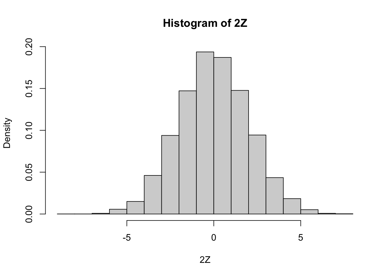
Estimate via simulation the pdf of \(\log\bigl(\left|Z\right|\bigr)\) when \(Z\) is standard normal.

expData <- log(abs(rnorm(10000)))
plot(density(expData),
     main = "Density of log|Z|",
     xlab = "log|Z|")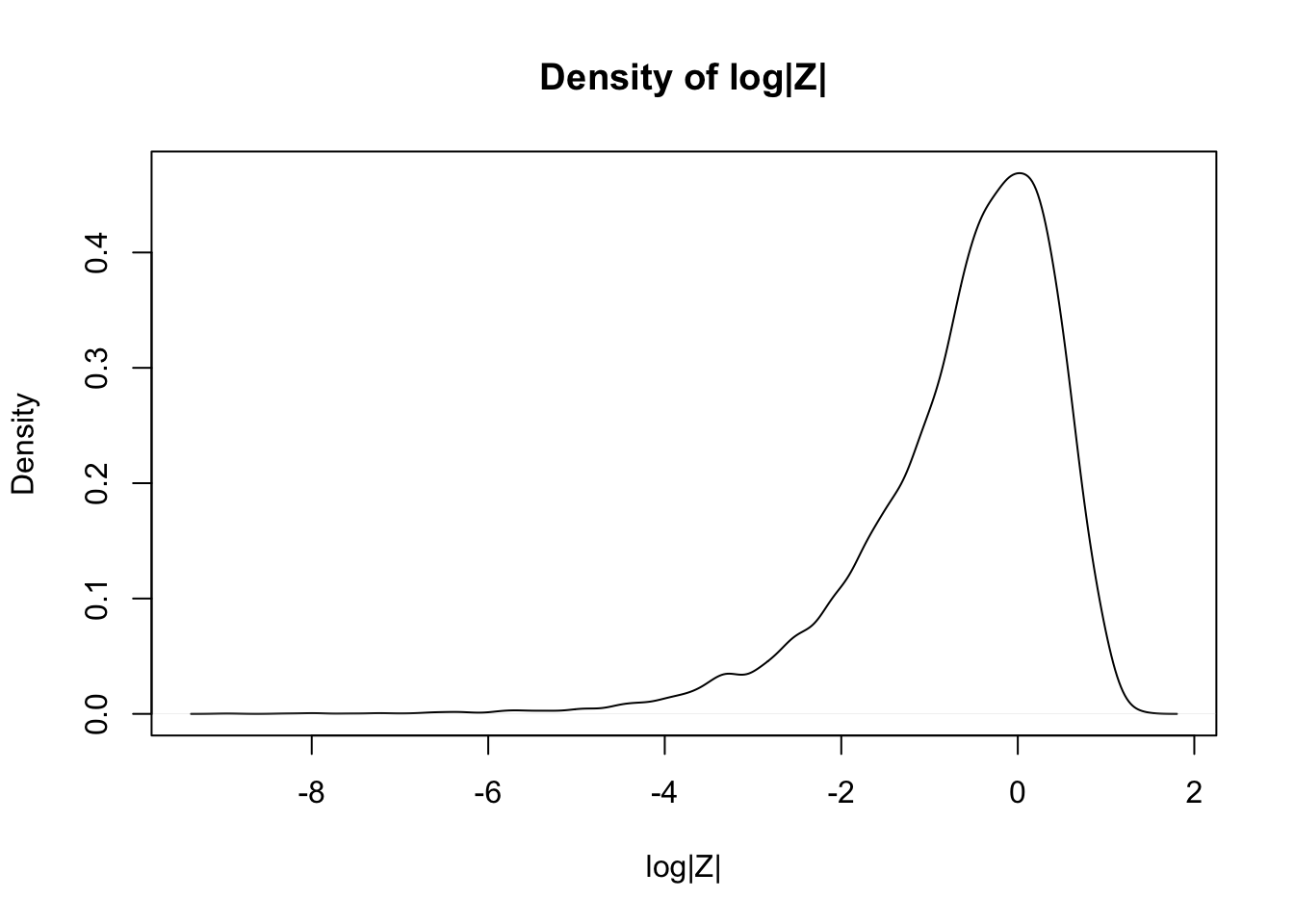

The simulations in Examples ?? and 1.10 worked well because the pdf of \(2Z\) and \(\log\bigl(\left|Z\right|\bigr)\) happen to be continuous functions. For pdfs with discontinuities, the density estimation tends to misleadingly smooth out the jumps in the function.

Example 1.11

Estimate the pdf of \(X\) when \(X\) is uniform on the interval \([-1,1]\).

unifData <- runif(10000,-1,1)
plot(density(unifData),
     main = "Density of Unif[-1,1]",
     xlab = "X")

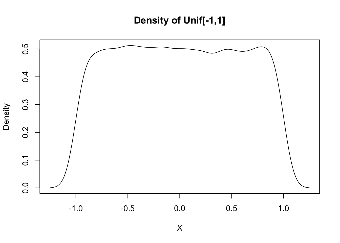
This distribution should be exactly 0.5 between -1 and 1, and zero everywhere else. The simulation is reasonable in the middle, but the discontinuities at the endpoints are not shown well. Increasing the number of data points helps, but does not fix the problem. Compare with the histogram approach, which seems to work better when the data comes from a distribution with a jump discontinuity.

hist(unifData, probability = TRUE,
     main = "Histogram of Unif[-1,1]",
     xlab = "X")

Example 1.12

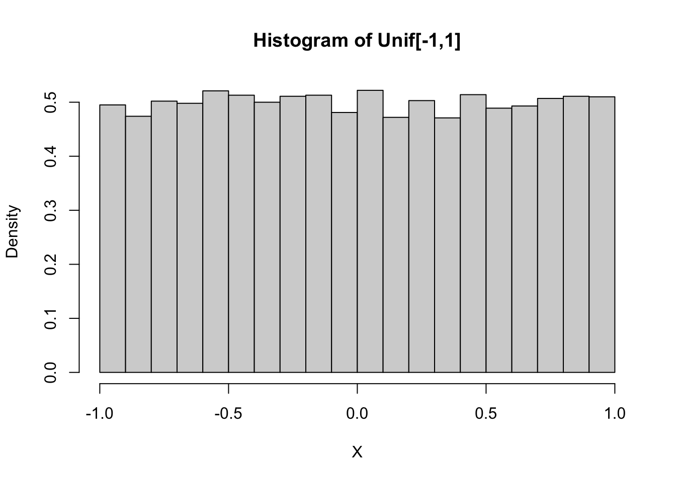
Estimate the pdf of \(X^2\) when \(X\) is uniform on the interval \([-1,1]\).

simdata <- replicate(10000, {
  unif_sample <- runif(1, -1, 1)
  unif_sample^2
})
plot(density(simdata),
     main = "Density of Uniform Squared",
     xlab = "X^2")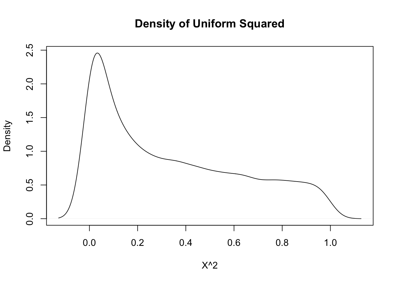

Example 1.13

Estimate the pdf of \(X + Y\) when \(X\) and \(Y\) are exponential random variables with rate 2.

simdata <- replicate(10000, {
  x <- rexp(1, 2)
  y <- rexp(1, 2)
  x + y
})
hist(simdata, probability = TRUE,
     main = "Histogram of Sum of Exponentials",
     xlab = "X + Y")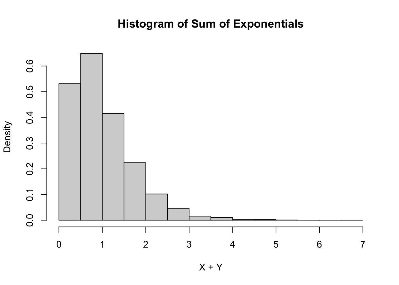

Example 1.14

Estimate the density of \(X_1 + X_2 + \cdots + X_{20}\) when all of the \(X_i\) are exponential random variables with rate 2.

This one is trickier and the first one for which it is significantly easier to use replicate to create the data. Let’s build up the experiment that we are replicating from the ground up.

Here’s the experiment of summing 20 exponential rvs with rate 2:

sum(rexp(20,2))

## [1] 3.436337

Now replicate it (10 times to test):

replicate(10, sum(rexp(20,2)))

##  [1] 12.214462 10.755431 13.170513  4.983875 10.259718  7.937500
##  [7] 11.313176 10.192818  7.386954 10.748529

Of course, we don’t want to just replicate it 10 times, we need about 10,000 data points to get a good density estimate.

sumExpData <- replicate(10000, sum(rexp(20,2)))
plot(density(sumExpData),
     main = "Density of Sum of 20 Exponentials",
     xlab = "X1 + ... + X20")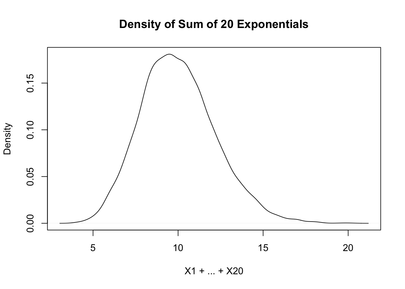

Note that this is starting to look like a normal random variable!!

Theorems about transformations of random variables

In this section, we will be estimating the pdf of transformations of random variables and comparing them to known pdfs. The goal is to find a known pdf that closely matches our estimate, so that we can develop some relationships between common rvs.

Example 1.15

Compare the pdf of \(2Z\), where \(Z\sim \text{Normal}(0,1)\) to the pdf of a normal random variable with mean 0 and standard deviation 2.

We already saw how to estimate the pdf of \(2Z\), we just need to plot the pdf of \(\text{Normal}(0,2)\) on the same graph<sup>17</sup>. We show how to do this using both the histogram and the density plot approach. The pdf \(f(x)\) of \(\text{Normal}(0,2)\) is given in R by the function \(f(x) = \text{dnorm}(x,0,2)\).

zData <- 2 * rnorm(10000)
hist(zData, probability = TRUE,
     main = "Density and Histogram of 2Z",
     xlab = "2Z")
curve(dnorm(x, 0, 2), add = T)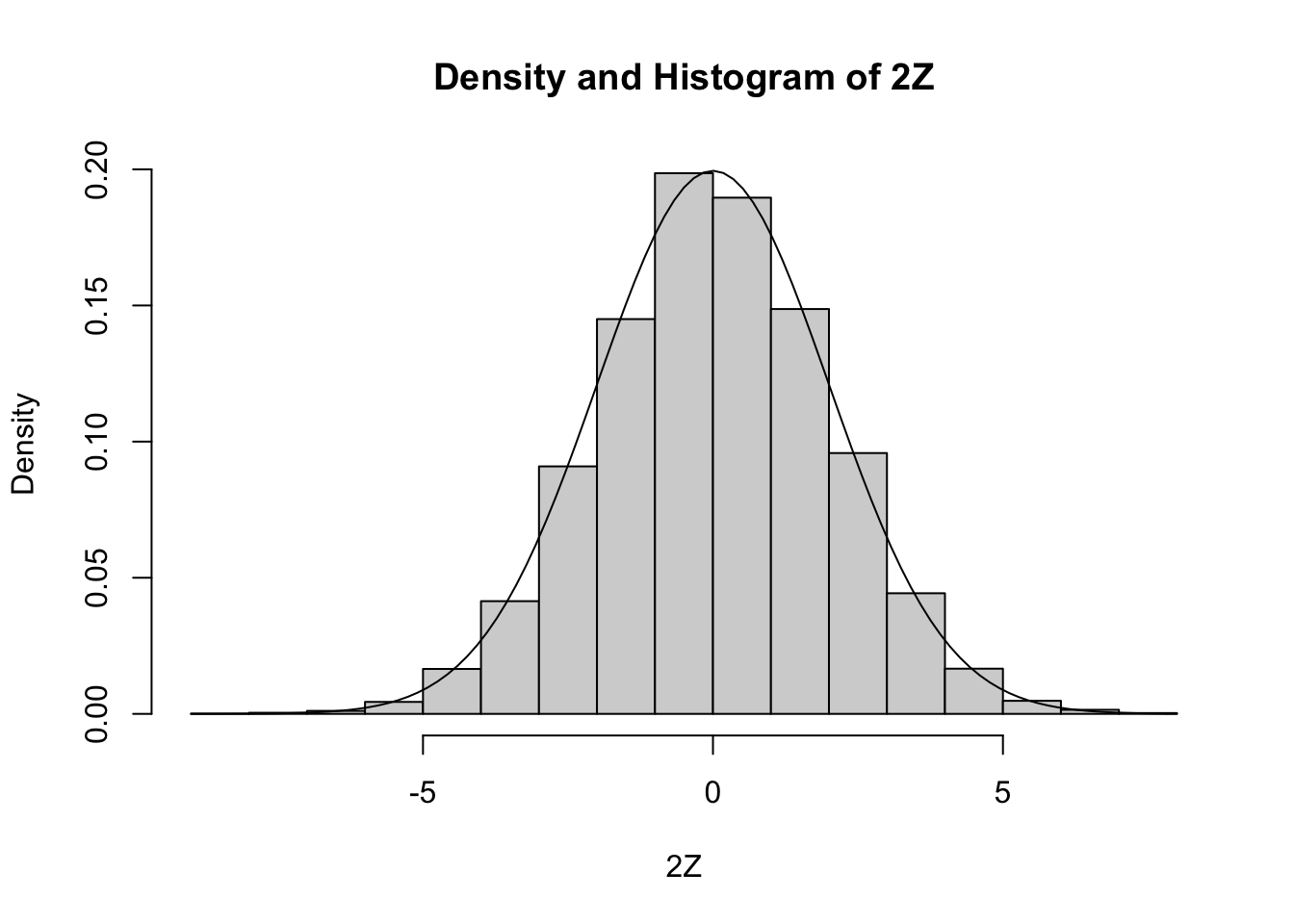

Since the area under of each rectangle in the histogram is approximately the same as the area under the curve over the same interval, this is evidence that \(2Z\) is normal with mean 0 and standard deviation 2. Next, let’s look at the density estimation together with the true pdf of a normal with mean 0 and \(\sigma = 2\).

plot(density(zData), 
     xlab = "2Z", 
     main = "Density 2Z and Normal(0, 2)")
curve(dnorm(x, 0, 2), add = T, col = 2)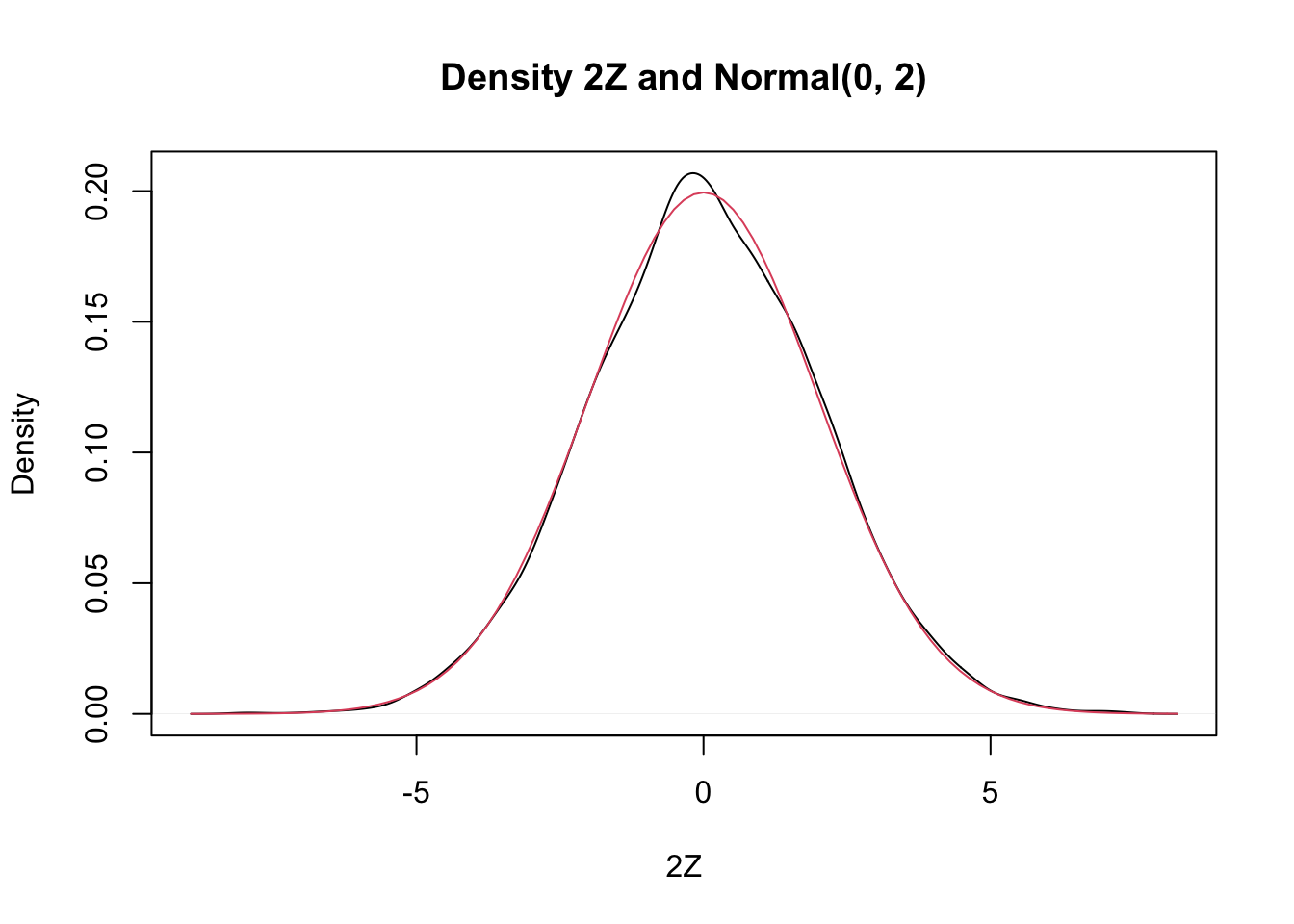

Wow! Those look really close to the same thing! This is again evidence that \(2Z \sim \text{Normal}(0, 2)\). It would be a good idea to label the red curve and the black curve. This kind of thing is typically easier using ggplot2, which will be discussed in Chapter 4.

Theorem 1.1

Let \(X\) be a normal random variable with mean \(\mu\) and standard deviation \(\sigma\). Then, \(aX + b\) is a normal random variable with mean \(a\mu + b\) and standard deviation \(a\sigma\).

Example 1.16

Let \(Z\) be a standard normal rv. Find the pdf of \(Z^2\) and compare it to the pdf of a \(\chi^2\) (chi-squared) rv with one degree of freedom. The distname for a \(\chi^2\) rv is chisq, and rchisq requires the degrees of freedom to be specified using the df parameter.

We plot the pdf of \(Z^2\) and the chi-squared rv with one degree of freedom on the same plot.

zData <- rnorm(10000)^2
hist(zData, 
     probability = T, 
     main = "Density and Histogram of Z^2",
     xlab = "Z^2")
curve(dchisq(x, df = 1), add = T)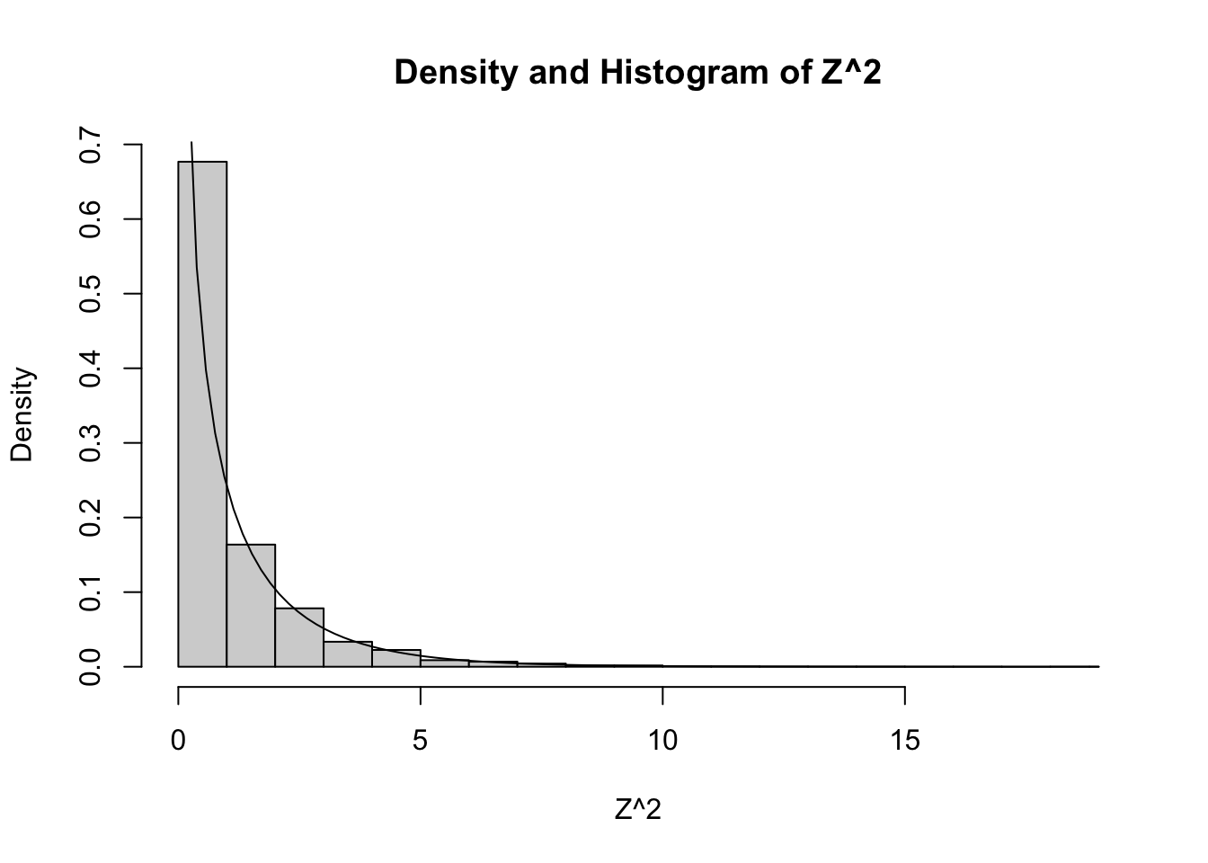

As you can see, the estimated density follows the true histogram quite well. This is evidence that \(Z^2\) is, in fact, chi-squared. Notice that \(\chi^2\) with one df has a vertical asymptote at \(x = 0\).

Theorem 1.2

Let \(Z\) be a normal random variable with mean 0 and standard deviation 1. Then, \(Z^2\) is a chi-squared random variable with 1 degree of freedom.

The Central Limit Theorem

Definition 1.17

Random variables \(X_1,\ldots,X_n\) are called independent identically distributed or iid if each pair of variables are independent, and each \(X_i\) has the same probability distribution.

All of the r + distname functions (rnorm, rexp, etc.) produce iid random variables. In the real world, iid rvs are produced by randomly sampling a population. As long as the population size is much larger than \(n\), the sampled values will be independent, and all will have the same probability distribution as the population distribution. In practice, it is quite hard to sample randomly from a real population.

Combining iid random variables can produce random variables with known distributions, even if the population being sampled is unknown. An example of this phenomenon is the Central Limit Theorem, which is fundamental to statistical reasoning.

In its most straightforward version, the Central Limit Theorem is a statement about the mean of the variables \(X_1,\ldots,X_n\), the random variable \(\overline{X}\):

\[ \overline{X} = \frac{X_1 + \dotsb + X_n}{n}. \]

We call \(\overline{X}\) the sample mean because it is the mean of a random sample.

Theorem 1.3 (Central Limit Theorem)

Let \(X_1,\ldots,X_n\) be iid rvs with finite mean \(\mu\) and standard deviation \(\sigma\). Then \[ \frac{\overline{X} - \mu}{\sigma/\sqrt{n}} \to Z \qquad \text{as}\ n \to \infty \] where \(Z\) is a standard normal rv.

We will not prove Theorem 1.3, but we will do simulations for several examples. They will all follow a similar format.

Example 1.18

Let \(X_1,\ldots,X_{30}\) be Poisson random variables with rate 2. From our knowledge of the Poisson distribution, each \(X_i\) has mean \(\mu = 2\) and standard deviation \(\sigma = \sqrt{2}\). The central limit theorem says that \[ \frac{\overline{X} - 2}{\sqrt{2}/\sqrt{30}} \] will be approximately normal with mean 0 and standard deviation 1 if \(n = 30\) is a large enough sample size. We will investigate later how to determine what a large enough sample size would be, but for now we assume that for this case, \(n = 30\) is big enough. Let us check this with a simulation.

This is a little but more complicated than our previous examples, but the idea is still the same. We create an experiment which computes \(\overline{X}\) and then transforms by subtracting 2 and dividing by \(\sqrt{2}/\sqrt{30}\).

Here is a single experiment:

xbar <- mean(rpois(30,2))
(xbar - 2)/(sqrt(2)/sqrt(30))

## [1] 0.9036961

Now, we replicate and plot:

poisData <- replicate(10000, {
  xbar <- mean(rpois(30,2))
  (xbar - 2)/(sqrt(2)/sqrt(30))
})
plot(density(poisData), 
     main = "Standardized sum of Poisson Compared to Normal",
     xlab = "x")
curve(dnorm(x), add = T, col = 2)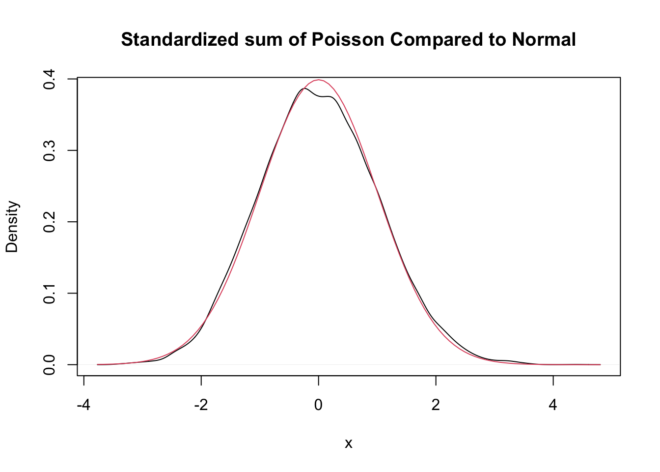

Very close!

Example 1.19

Let \(X_1,\ldots,X_{50}\) be exponential random variables with rate 1/3. From our knowledge of the exponential distribution, each \(X_i\) has mean \(\mu = 3\) and standard deviation \(\sigma = 3\). The central limit theorem says that \[ \frac{\overline{X} - 3}{3/\sqrt{n}} \] is approximately normal with mean 0 and standard deviation 1 when \(n\) is large. We check this with a simulation in the case \(n = 50\). Again, we can either use histograms or density estimates for this, but this time we choose to use density estimates.

expData <- replicate(10000, {
  dat <- mean(rexp(50,1/3))
  (dat - 3)/(3/sqrt(50))
})
plot(density(expData), 
     main = "Standardized sum of exponentials compared to normal",
     xlab = "x")
curve(dnorm(x), add = T, col = 2)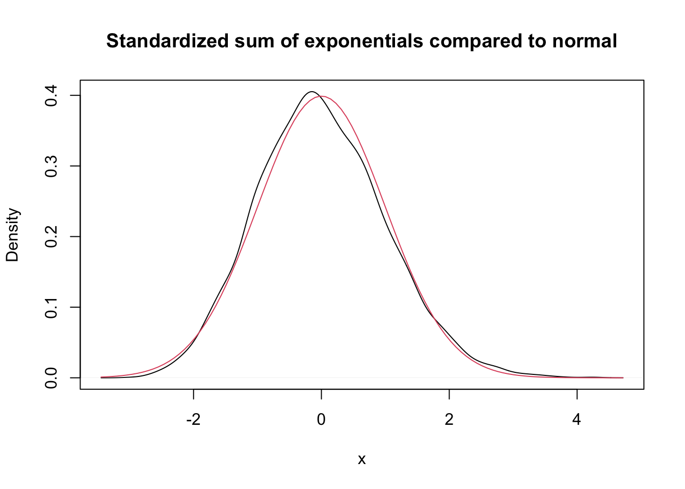

The Central Limit Theorem says that, if you take the mean of a large number of independent samples, then the distribution of that mean will be approximately normal. How large does \(n\) need to be in practice?

• If the population you are sampling from is symmetric with no outliers, a good approximation to normality appears after as few as 15-20 samples.
• If the population is moderately skew, such as exponential or \(\chi^2\), then it can take between 30-50 samples before getting a good approximation.
• Data with extreme skewness, such as some financial data where most entries are 0, a few are small, and even fewer are extremely large, may not be appropriate for the central limit theorem even with 500 samples (see Example 1.20).

There are versions of the Central Limit Theorem available when the \(X_i\) are not iid, but outliers of sufficient size will cause the distribution of \(\overline{X}\) to not be normal, see Exercise 1.27.

Example 1.20

A distribution for which sample size of \(n = 500\) is not sufficient for good approximation via normal distributions.

We create a distribution that consists primarily of zeros, but has a few modest sized values and a few large values:

# Start with lots of zeros
skewdata <- replicate(2000,0)
# Add a few moderately sized values
skewdata <- c(skewdata, rexp(200,1/10))
# Add a few large values
skewdata <- c(skewdata, seq(100000,500000,50000))

mu <- mean(skewdata)
sig <- sd(skewdata)

We use sample to take a random sample of size \(n\) from this distribution. We take the mean, subtract the true mean of the distribution, and divide by \(\sigma/\sqrt{n}\). We replicate that 10000 times. Here are the plots when \(\overline{X}\) is the mean of 100 samples:

n <- 100

skewSample <- replicate(10000, {
  dat <- mean(sample(skewdata, n, TRUE)) 
  (dat - mu)/(sig/sqrt(n))
})
hist(skewSample, probability = T,
     main = "Histogram of Standardized Mean of 100 Samples",
     xlab = "X")
curve(dnorm(x), add = T, col = 2)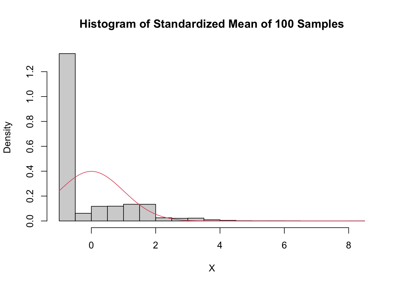

and 500 samples:

n <- 500

skewSample <- replicate(10000, {
  dat <- mean(sample(skewdata, n, TRUE)) 
  (dat - mu)/(sig/sqrt(n))
})

hist(skewSample, probability = T,
     main = "Histogram of Standardized Mean of 500 Samples",
     xlab = "x")
curve(dnorm(x), add = T, col = 2)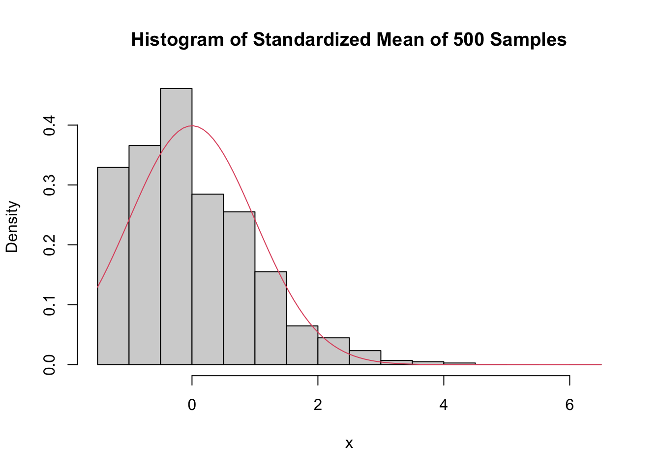

Even at 500 samples, the density is still far from the normal distribution, especially the lack of left tail. Of course, the Central Limit Theorem is still true, so \(\overline{X}\) must become normal if we choose \(n\) large enough:

n <- 5000

skewSample <- replicate(10000, {
  dat <- mean(sample(skewdata, n, TRUE)) 
  (dat - mu)/(sig/sqrt(n))
})

hist(skewSample, probability = T,
     main = "Histogram of Standardized Mean of 5000 Samples",
     xlab = "x")
curve(dnorm(x), add = T, col = 2)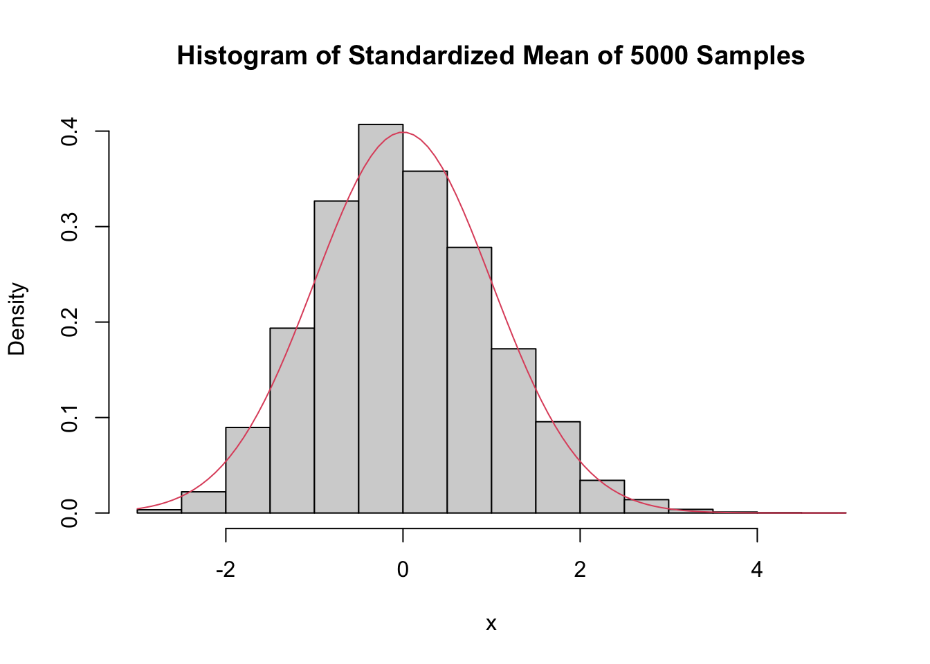

There may still be a slight skewness in this picture, but it is finally close to normal.

Sampling Distributions

We describe \(t\), \(\chi^2\) and \(F\) in the context of samples from normal rv. Emphasis is on understanding relationship between the rv and how it comes about from \(\overline{X}\) and \(S\). The goal is for you not to be surprised when we say later that test statistics have certain distributions. You may not be able to prove it, but hopefully won’t be surprised either. We’ll use density estimation extensively to illustrate the relationships.

Definition 1.21

Assume \(X_1,\ldots,X_n\) are independent and identically distributed with mean \(\mu\) and standard deviation \(\sigma\). Define:

• The sample mean \[ \overline{X} = \sum_{i=1}^n X_i \]
• The sample variance \[ S^2 = \frac 1{n-1} \sum_{i=1}^n (X_i - \overline{X})^2 \]
• The sample standard deviation is \(S\), the square root of the sample variance.

We note that \(\overline{X}\) is an estimator for \(\mu\) and \(S\) is an estimator for \(\sigma\).

Linear combination of normal rv’s

Let \(X_1,\ldots,X_n\) be rvs with means \(\mu_1,\ldots,\mu_n\) and variances \(\sigma_i^2\). Then by Theorem 5.8 \[ E[\sum a_i X_i] = \sum a_i E[X_i] \] and if \(X_1, \ldots, X_n\) are independent, then by Theorem 5.10 \[ V(\sum a_i X_i) = \sum a_i^2 V(X_i) \] As a consequence, \(E[aX + b] = aE[X] + b\) and \(V(aX + b) = a^2V(X)\). An important special case is that if \(X_1,\ldots,X_n\) are iid with mean \(\mu\) and variance \(\sigma^2\), then \(\overline{X}\) has mean \(\mu\) and variance \(\sigma^2/n\).

In the special case that \(X_1,\ldots, X_n\) are iid normal random variables, much more can be said. The following theorem generalizes our previous result to sums of more than two random variables.

Theorem 1.4

Let \(X_1,\ldots,X_n\) be independent normal rvs with means \(\mu_1,\ldots,\mu_n\) and variances \(\sigma_1^2,\ldots,\sigma_n^2\). Then, \[ \sum_{i=1}^n a_i X_i \] is normal with mean \(\sum a_i \mu_i\) and variance \(\sum a_i^2 \sigma_i^2\).

You will be asked to verify this via estimating densities in special cases in the exercises. The special case that is very interesting is the following:

Theorem 1.5

Let \(X_1,\ldots,X_n\) be independent identically distributed normal rvs with common mean \(\mu\) and variance \(\sigma^2\). Then \[ \frac{\overline{X} - \mu}{\sigma/\sqrt{n}} \] is standard normal(0,1).

Chi-squared

Definition 1.22

Let \(Z\) be a standard normal random variable. An rv with the same distribution is \(Z^2\) is called a Chi-squared random variable with one degree of freedom.

Let \(Z_1, \dotsc, Z_n\) be \(n\) iid standard normal random variables. Then an rv with the same distribution as \(Z_1^2 + \dotsb + Z_n^2\) is called a Chi-squared random variable with \(n\) degrees of freedom.

Remark

The sum of \(n\) independent \(\chi^2\) rv’s with 1 degree of freedom is a \(\chi^2\) rv with \(n\) degrees of freedom. More generally, the sum of a \(\chi^2\) with \(\nu_1\) degrees of freedom and a \(\chi^2\) with \(\nu_2\) degrees of freedom is \(\chi^2\) with \(\nu_1 + \nu_2\) degrees of freedom.

Let’s check by estimating pdfs that the sum of a \(\chi^2\) with 2 df and a \(\chi^2\) with 3 df is a \(\chi^2\) with 5 df.

chi2Data <- replicate(10000, rchisq(1,2) + rchisq(1,3))
hist(chi2Data, probability = TRUE,
     main = "Histogram of sum of Chi^2 Random Variables",
     xlab = "x + y")
curve(dchisq(x, df = 5), add = T, col = 2)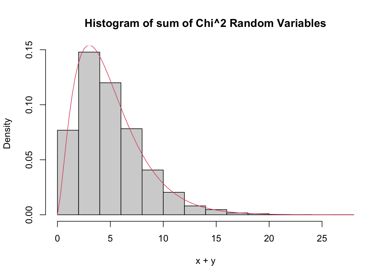

The \(\chi^2\) distribution is important for understanding the sample standard deviation.

Theorem 1.6

If \(X_1,\ldots,X_n\) are iid normal rvs with mean \(\mu\) and standard deviation \(\sigma\), then \[ \frac{n-1}{\sigma^2} S^2 \] has a \(\chi^2\) distribution with \(n-1\) degrees of freedom.

We provide a heuristic and a simulation as evidence that Theorem 1.6 is true. Additionally, in Exercise 1.32 you are asked to prove Theorem 1.6 in the case that \(n = 2\).

Heuristic argument: Note that \[ \frac{n-1}{\sigma^2} S^2 = \frac 1{\sigma^2}\sum_{i=1}^n (X_i - \overline{X})^2 \\ = \sum_{i=1}^n \bigl(\frac{X_i - \overline{X}}{\sigma}\bigr)^2 \] Now, if we had \(\mu\) in place of \(\overline{X}\) in the above equation, we would have exactly a \(\chi^2\) with \(n\) degrees of freedom. Replacing \(\mu\) by its estimate \(\overline{X}\) reduces the degrees of freedom by one, but it remains \(\chi^2\).

For the simulation, we estimate the density of \(\frac{n-1}{\sigma^2} S^2\) and compare it to that of a \(\chi^2\) with \(n-1\) degrees of freedom, in the case that \(n = 4\), \(\mu = 3\) and \(\sigma = 9\).

sdData <- replicate(10000, 3/81 * sd(rnorm(4, 3, 9))^2)
hist(sdData, probability = TRUE,
     main = "Histogram of Sample Variance Compared to Chi^2",
     xlab = "S",
     ylim = c(0, .25))
curve(dchisq(x, df = 3), add = T, col = 2)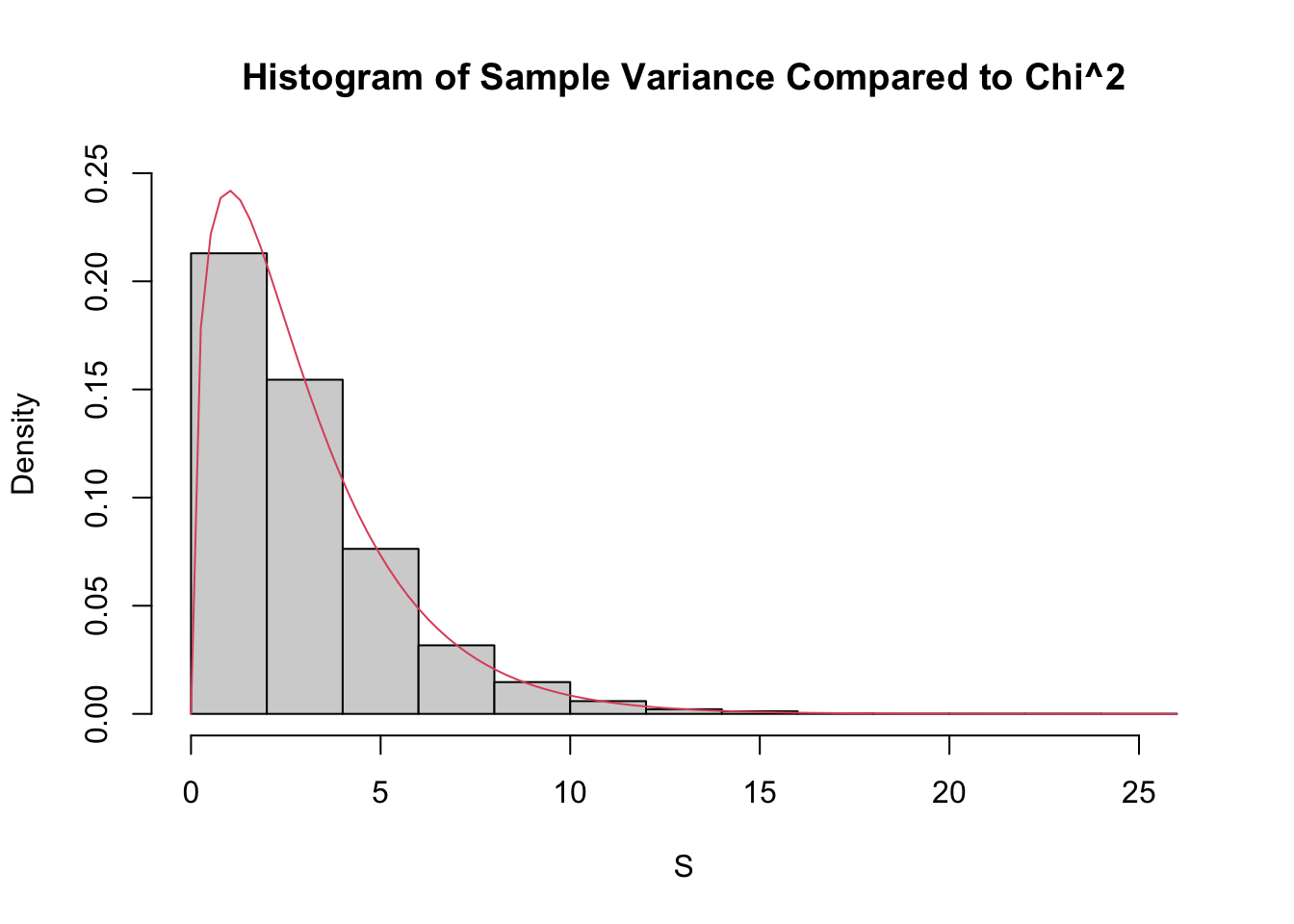

The \(t\) distribution

Definition 1.23

If \(Z\) is a standard normal(0,1) rv, \(\chi^2_\nu\) is a Chi-squared rv with \(\nu\) degrees of freedom, and \(Z\) and \(\chi^2_\nu\) are independent, then

\[ t_\nu = \frac{Z}{\sqrt{\chi^2_\nu/\nu}} \]

is distributed as a \(t\) random variable with \(\nu\) degrees of freedom.

Theorem 1.7

If \(X_1,\ldots,X_n\) are iid normal rvs with mean \(\mu\) and sd \(\sigma\), then \[ \frac{\overline{X} - \mu}{S/\sqrt{n}} \] is \(t\) with \(n-1\) degrees of freedom.

Note that \(\frac{\overline{X} - \mu}{\sigma/\sqrt{n}}\) is normal(0,1). So, replacing \(\sigma\) with \(S\) changes the distribution from normal to \(t\).

Proof:

\[ \frac{Z}{\sqrt{\chi^2_{n-1}/n}} = \frac{\overline{X} - \mu}{\sigma/\sqrt{n}}*\sqrt{\frac{\sigma^2 (n-1)}{S^2(n-1)}}\\ = \frac{\overline{X} - \mu}{S/\sqrt{n}} \] Where we have used that \((n - 1) S^2/\sigma^2\) is \(\chi^2\) with \(n - 1\) degrees of freedom.

Example 1.24

Estimate the pdf of \(\frac{\overline{X} - \mu}{S/\sqrt{n}}\) in the case that \(X_1,\ldots,X_6\) are iid normal with mean 3 and standard deviation 4, and compare it to the pdf of the appropriate \(t\) random variable.

tData <- replicate(10000, {
  normData <- rnorm(6,3,4)
  (mean(normData) - 3)/(sd(normData)/sqrt(6))
}) 
hist(tData, 
     probability = TRUE,
     ylim = c(0, .37),
     main = "Histogram of t",
     xlab = "t")
curve(dt(x, df = 5), add = TRUE, col = 2)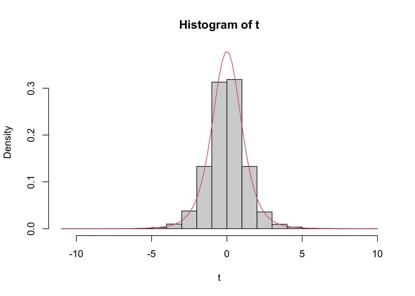

We see a very good agreement.

The F distribution

An \(F\) distribution has the same density function as \[ F_{\nu_1, \nu_2} = \frac{\chi^2_{\nu_1}/\nu_1}{\chi^2_{\nu_2}/\nu_2} \] We say \(F\) has \(\nu_1\) numerator degrees of freedom and \(\nu_2\) denominator degrees of freedom.

One example of this type is: \[ \frac{S_1^2/\sigma_1^2}{S_2^2/\sigma_2^2} \] where \(X_1,\ldots,X_{n_1}\) are iid normal with standard deviation \(\sigma_1\) and \(Y_1,\ldots,Y_{n_2}\) are iid normal with standard deviation \(\sigma_2.\)

Summary

1. \(aX+ b\) is normal with mean \(a\mu + b\) and standard deviation \(a\sigma\) if \(X\) is normal with mean \(\mu\) and sd \(\sigma\).
2. \(\frac{X - \mu}{\sigma}\sim Z\) if \(X\) is Normal(\(\mu, \sigma\)).
3. \(\frac{\overline{X} - \mu}{\sigma/\sqrt{n}} \sim Z\) if \(X_1,\ldots,X_n\) iid normal(\(\mu, \sigma\))
4. \(\lim_{n\to \infty} \frac{\overline{X} - \mu}{\sigma/\sqrt{n}} \sim Z\) if \(X_1,\ldots,X_n\) iid with finite variance.
5. \(Z^2 \sim \chi^2_1\)
6. \(\chi^2_\nu + \chi^2_\eta \sim \chi^2_{\nu + \eta}\)
7. \(\frac{(n-1)S^2}{\sigma^2} \sim \chi^2_{n-1}\) when \(X_1,\ldots,X_n\) iid normal.
8. \(\frac Z{\sqrt{\chi^2_\nu/\nu}} \sim t_\nu\)
9. \(\frac{\overline{X} - \mu}{S/\sqrt{n}}\sim t_{n-1}\) when \(X_1,\ldots,X_n\) iid normal.
10. \(\frac{\chi^2_\nu/\nu}{\chi^2_\mu/\mu} \sim F_{\nu, \mu}\)
11. \(\frac{S_1^2/\sigma_1^2}{S_2^2/\sigma_2^2} \sim F_{n_1 - 1, n_2 - 1}\) if \(X_1,\ldots,X_{n_1}\) iid normal with sd \(\sigma_1\) and \(Y_1,\ldots,Y_{n_2}\) iid normal with sd \(\sigma_2\).

Point Estimators

Suppose that a random variable \(X\) depends on some parameter \(\beta\). In many instances we do not know \(\beta\), but are interested in estimating it from observations of \(X\) or from data. Formally, if \(X_1, \ldots, X_n\) are iid with the same distribution as \(X\), then a point estimator is a function \(h(X_1, \ldots, X_n)\). Normally, the value of \(h(X_1, \ldots, X_n)\) represents our best guess as to what the parameter \(\beta\) is, based on the data. We write \(\hat \beta = h(X_1, \ldots, X_n)\) for the point estimator of \(\beta\), and we note that \(\hat \beta\) is a random variable.

For example, if \(X\) is a normal rv with unknown mean \(\mu\), and we get data \(X_1,\ldots, X_n\), it would be very natural to estimate \(\mu\) by \(\frac 1n \sum_{i=1}^n X_i\). Notationally, we say \[ \hat \mu = \frac 1n \sum_{i=1}^n X_i = \overline{X} \] In other words, our estimate of \(\mu\) from the data \(x_1,\ldots, x_n\) is denoted by \(\hat \mu\).

The two point estimators that we are interested in in this section are point estimators for the mean of an rv and the variance of an rv. (Note that we have switched gears a little bit, because the mean and variance aren’t necessarily parameters of the rv. We are really estimating functions of the parameters at this point. The distinction will not be important for the purposes of this text.)

Recall that the definition of the mean of a discrete rv with possible values \(x_i\) is \[ E[X] = \mu = \sum_{i=1}^n x_i p(x_i) \] If we are given data \(x_1,\ldots,x_n\), it is natural to assign \(p(x_i) = 1/n\) for each of those data points to create a new random variable \(X_0\), and we obtain \[ E[X_0] = \frac 1n \sum_{i=1}^n x_i = \overline{x} \] This is a natural choice for our point estimator for the mean of the rv \(X\), as well. \[ \hat \mu = \overline{x} = \frac 1n \sum_{i=1}^n x_i \]

Continuing in the same way, if we are given data \(x_1,\ldots,x_n\) and we wish to estimate the variance, then we could create a new random variable \(X_0\) whose possible outcomes are \(x_1,\ldots,x_n\) with probabilities \(1/n\), and compute \[ \sigma^2 = E[(X- \mu)^2] = \frac 1n \sum_{i=1}^n (x_i - \mu)^2 \] This works just fine as long as \(\mu\) is known. However, most of the time, we do not know \(\mu\) and we must replace the true value of \(\mu\) with our estimate from the data. There is a heuristic that each time you replace a parameter with an estimate of that parameter, you divide by one less. Following that heuristic, we obtain \[ \hat \sigma^2 = S^2 = \frac 1{n-1} \sum_{i=1}^n (x_i - \overline{x})^2 \]

Properties of Point Estimators

The point estimators for \(\mu\) and \(\sigma^2\) are random variables themselves, since they are computed from a random sample from a distribution. As such, they also have distributions, means and variances. One property of point estimators that is often desirable is that it is unbiased.

Definition 1.25

A point estimator \(\hat \beta\) for \(\beta\) is an unbiased estimator if \(E[\hat \beta] = \beta\).

Intuitively, “unbiased” means that the estimator does not consistently underestimate or overestimate the parameter it is estimating. If we were to estimate the parameter over and over again, the average value of the estimates would converge to the correct value of the parameter.

Let’s consider \(\overline{x}\) and \(S^2\). Are they unbiased? It is possible to determine this analytically, and interested students should consult Wackerly<sup>18</sup> for a proof. However, we will do this using R and simulation.

Example 1.26

Let \(X_1,\ldots, X_{5}\) be a random sample from a normal distribution with mean 1 and variance 1. Compute \(\overline{x}\) based on the random sample.

mean(rnorm(5,1,1))

## [1] 1.614421

You can see the estimate is pretty close to the correct value of 1, but not exactly 1. However, if we repeat this experiment 10,000 times and take the average value of \(\overline{x}\), that should be very close to 1.

mean(replicate(10000, mean(rnorm(5,1,1))))

## [1] 1.003684

It can be useful to repeat this a few times to see whether it seems to be consistently overestimating or underestimating the mean. In this case, it is not.

Example 1.27

Let \(X_1,\ldots,X_5\) be a random sample from a normal rv with mean 1 and variance 4. Estimate the variance using \(S^2\).

sd(rnorm(5,1,2))^2

## [1] 5.398046

We see that our estimate is not ridiculous, but not the best either. Let’s repeat this 10,000 times and take the average. (We are estimating \(E[S^2]\).)

mean(replicate(10000, sd(rnorm(5,1,2))^2))

## [1] 3.986978

Again, repeating this a few times, it seems that we are neither overestimating nor underestimating the value of the variance.

Example 1.28

The formula for \(S^2\), the sample variance, contains a division by \(n-1\), even though the sum has \(n\) terms. In this example, we see that dividing by \(n\) would lead to a biased estimator.

That is, \(\frac 1n \sum_{i=1}^n (x_i - \overline{x})^2\) is not an unbiased estimator of \(\sigma^2\).

We use replicate twice. On the inside, it is running 10000 simulations. On the outside, it is repeating the overall simulation 8 times.

replicate(8,
  mean(replicate(10000, {
    data = rnorm(5,1,2) 
    1/5*sum((data - mean(data))^2)
  }))
)

## [1] 3.242466 3.212477 3.231688 3.187677 3.157526 3.218117 3.227146
## [8] 3.159302

In each of the 8 trials, \(\frac 1n \sum_{i=1}^n (x_i - \overline{x})^2\) underestimates the correct value \(\sigma^2 = 4\) by quite a bit.

Variance of Unbiased Estimators

From the above, we can see that \(\overline{x}\) and \(S^2\) are unbiased estimators for \(\mu\) and \(\sigma^2\), respectively. There are other unbiased estimator for the mean and variance, however. For example, if \(X_1,\ldots,X_n\) is a random sample from a normal rv, then the median of the \(X_i\) is also an unbiased estimator for the mean. Moreover, the median seems like a perfectly reasonable thing to use to estimate \(\mu\), and in many cases is actually preferred to the mean. There is one way, however, in which the sample mean \(\overline{x}\) is definitely better than the median, and that is that it has a lower variance. So, in theory at least, \(\overline{x}\) should not deviate from the true mean as much as the median will deviate from the true mean, as measured by variance.

Let’s do a simulation to illustrate. Suppose you have a random sample of size 11 from a normal rv with mean 0 and standard deviation 1. We estimate the variance of \(\overline{x}\).

sd(replicate(10000, mean(rnorm(11,0,1))))^2

## [1] 0.09039206

Now we repeat for the median.

sd(replicate(10000, median(rnorm(11,0,1))))^2

## [1] 0.1376239

And, we see that the variance of the mean is lower than the variance of the median. This is a good reason to use the sample mean to estimate the mean of a normal rv rather than using the median, absent other considerations such as outliers.

Vignette: Loops in R

Most tasks in R can be done using the implicit loops described in this section. There are also powerful tools in the purrr package. However, sometimes it is easiest just to write a conventional loop. This vignette explains how to use while loops in the context of simulations.

As a warm-up, let’s estimate the expected value of the number of tosses of a fair coin before the first time Heads occurs. We had been doing this type of problem by assuming that we will always get Heads before, say, the 100th toss. That seems safe in this context, but we can’t always replace an experiment that could take arbitrarily many steps to complete with one that has a maximum number of steps. We will use a while loop to do this instead.

A while loop repeats one or more statements until a certain condition is no longer met. It is crucial when writing a while loop that you ensure that the condition to exit the loop will eventually be satisfied! The format looks like this.

i <- 0 #initialize
while(i < 2) { #check condition
  print(i)
  i <- i + 1 #increment
}

## [1] 0
## [1] 1

R sets i to 0 and then checks whether i < 2 (it is). It then prints i and adds one to i. It checks again - is i < 2? Yes, so it prints i and adds one to it. At this point i is not less than 2, so R exits the loop. Now, let’s set up a while loop that counts the number of Tails before the first Head.

num_tails <- 0
coin_toss <- sample(c("Head", "Tail"), 1)
if(coin_toss == "Tail") {
  num_tails <- num_tails + 1
}
while(coin_toss != "Head") {
  coin_toss <- sample(c("Head", "Tail"), 1)
  if(coin_toss == "Tail") {
    num_tails <- num_tails + 1
  }
}
num_tails

## [1] 1

So, if we wanted to simulate the number of tails before the first head, we could put replicate around the above code, just like we always do.

sim_data <- replicate(1000, {
  num_tails <- 0
  coin_toss <- sample(c("Head", "Tail"), 1)
  if(coin_toss == "Tail") {
    num_tails <- num_tails + 1
  }
  while(coin_toss != "Head") {
    coin_toss <- sample(c("Head", "Tail"), 1)
    if(coin_toss == "Tail") {
      num_tails <- num_tails + 1
    }
  }
  num_tails
})
mean(sim_data)

## [1] 1.086

We get that the mean is about 1, which agrees with what we already knew.

Exercises

---

Exercises 1.2 - 1.3 require material through Section ??.

1.2

Let \(Z\) be a standard normal random variable. Estimate via simulation \(P(Z^2 < 2)\).

1.3

Let \(X\) and \(Y\) be independent exponential random variables with rate 3. Let \(Z = \max(X, Y)\) be the maximum of \(X\) and \(Y\). a. Estimate via simulation \(P(Z < 1/2)\). b. Estimate the mean and standard deviation of \(Z\).

---

Exercises 1.4 - 1.12 require material through Section ??.

1.4

Five coins are tossed and the number of heads \(X\) is counted. Estimate via simulation the pmf of \(X\).

1.5

Three dice are tossed and their sum \(X\) is observed. Use simulation to estimate and plot the pmf of \(X\).

1.6

Five six-sided dice are tossed and their product is observed. Use the estimated pmf to find the most likely outcome.

1.7

Fifty people put their names in a hat. They then all randomly choose one name from the hat. Let \(X\) be the number of people who get their own name. Estimate and plot the pmf of \(X\).

1.8

Consider an experiment where 20 balls are placed randomly into 10 urns. Let \(X\) denote the number of urns that are empty.

1. Estimate via simulation the pmf of \(X\).
2. What is the most likely outcome?
3. What is the least likely outcome that has positive probability?

1.9 (Hard)

Suppose 6 people, numbered 1-6, are sitting at a round dinner table with a big plate of spaghetti, and a bag containing 5005 red marbles and 5000 blue marbles. Person 1 takes the spaghetti, serves themselves, and chooses a marble. If the marble is red, they pass the spaghetti to the left. If it is blue, they pass the spaghetti to the right. The guests continue doing this until the last person receives the plate of spaghetti. Let \(X\) denote the number of the person holding the spaghetti at the end of the experiment. Estimate the pmf of \(X\).

1.10

Suppose you roll a die until the first time you obtain an even number. Let \(X_1\) be the total number of times you roll a 1, and let \(X_2\) be the total number of times that you roll a 2.

1. Is \(E[X_1] = E[X_2]\)? (Hint: Use simulation. It is extremely unlikely that you will roll 30 times before getting the first even number, so you can safely assume that the first even occurs inside of 30 rolls.)
2. Is the pmf of \(X_1\) the same as the pmf of \(X_2\)?
3. Estimate the variances of \(X_1\) and \(X_2\).

1.11

Recall the Example 1.8 in the text, where we show that the most likely number of times you have more Heads than Tails when a coin is tossed 100 times is zero. Suppose you toss a coin 100 times.

1. Let \(X\) be the number of times in the 100 tosses that you have exactly the same number of Heads as Tails. Estimate the expected value of \(X\).
2. Let \(Y\) be the number of tosses for which you have more Heads than Tails. Estimate the expected value of \(Y\).

1.12

Suppose there are two candidates in an election. Candidate A receives 52 votes and Candidate B receives 48 votes. You count the votes one at a time, keeping a running tally of who is ahead. At each point, either A is ahead, B is ahead or they are tied. Let \(X\) be the number of times that Candidate B is ahead in the 100 tallies.

1. Estimate the pmf of \(X\).
2. Estimate \(P(X > 50)\).

---

Exercises 1.13 - 1.15 require material through Section ??.

1.13

Let \(X\) and \(Y\) be uniform random variables on the interval \([0,1]\). Estimate the pdf of \(X+Y\) and plot it.

1.14

Let \(X\) and \(Y\) be uniform random variables on the interval \([0,1]\). Let \(Z\) be the maximum of \(X\) and \(Y\).

1. Plot the pdf of \(Z\).
2. From your answer to (a), decide whether \(P(0 \le Z \le 1/3)\) or \(P(1/3\le Z \le 2/3)\) is larger.

1.15

Estimate the value of \(a\) such that \(P(a \le Y \le a + 1)\) is maximized when \(Y\) is the maximum value of two exponential random variables with mean 2.

---

Exercises 1.16 - 1.21 require material through Section ??.

1.16

Is the product of two normal rvs normal? Estimate via simulation the pdf of the product of \(X\) and \(Y\), when \(X\) and \(Y\) are normal random variables with mean 0 and standard deviation 1. How can you determine whether \(XY\) is normal? Hint: you will need to estimate the mean and standard deviation.

1.17

The minimum of two exponential rv’s with mean 2 is an exponential rv. Use simulation to determine what the rate is.

1.18

The sum of two independent chi-squared rv’s with 2 degrees of freedom is either exponential or chi-squared. Which one is it? What is the parameter associated with your answer?

1.19

Let \(X\) and \(Y\) be independent uniform rvs on the interval \([0,1]\). Estimate via simulation the pdf of the maximum of \(X\) and \(Y\), and compare it to the pdf of a beta distribution with parameters shape1 = 2 and shape2 = 1. (Use dbeta().)

1.20

Estimate the density of the maximum of 7 uniform random variables on the interval \([0,1]\). This density is also beta; what are the parameters for the beta distribution?

1.21

If \(X_1, \ldots, X_7\) are iid uniform(0, 1) random variables, and let \(Y\) be the second largest of the \(X_1, \ldots, X_7\).

1. Estimate the pdf of \(Y\)
2. This pdf is also beta. What are the parameters?

---

Exercises 1.22 - 1.27 require material through Section ??.

1.22

Let \(X_1,\ldots,X_{n}\) be uniform rv’s on the interval \((0,1)\). How large does \(n\) need to be before the pdf of \(\frac{\overline{X} - \mu}{\sigma/\sqrt{n}}\) is approximately that of a standard normal rv? (Note: there is no “right” answer, as it depends on what is meant by “approximately.” You should try various values of \(n\) until you find one where the estimate of the pdf is close to that of a standard normal.)

1.23

Consider the Log Normal distribution, whose root in R is lnorm. The log normal distribution takes two parameters, meanlog and sdlog.

1. Graph the pdf of a Log Normal random variable with meanlog = 0 and sdlog = 1. The pdf of a Log Normal rv is given by dlnorm(x, meanlog, sdlog).
2. Let \(X\) be a log normal rv with meanlog = 0 and sdlog = 1. Estimate via simulation the density of \(\log(X)\), and compare it to a standard normal random variable.
3. Estimate the mean and standard deviation of a Log Normal random variable with parameters 0 and 1/2.
4. Using your answer from (b), find an integer \(n\) such that \[ \frac{\overline{X} - \mu}{\sigma/\sqrt{n}} \] is approximately normal with mean 0 and standard deviation 1.

1.24

Let \(X_1,\ldots,X_{n}\) be chi-squared rv’s with 2 degrees of freedom. How large does \(n\) need to be before the pdf of \(\frac{\overline{X} - \mu}{\sigma/\sqrt{n}}\) is approximately that of a standard normal rv? (Hint: it is not hard to find the mean and sd of chi-squared rvs on the internet.)

1.25

The Central Limit Theorem holds for the mean of iid random variables. For continuous random variables whose cdf’s have derivative greater than 0 at the median \(\theta\), the median is also approximately normal with mean \(\theta\) and standard deviation \(1/(2\sqrt{n}f(\theta))\) when the sample size is large. This exercise explores the normality of the median via simulations. The R function to compute the median of a sample is median.

1. Let \(X_1, \ldots, X_n\) be uniform random variables on \([-1, 1]\). The median is 0 and \(f(0) = 1/2\). Show that for large \(n\), the median of \(X_1, \ldots, X_n\) is approximately normal with mean 0 and standard deviation \(1/\sqrt{n}\).
2. Let \(X_1, \ldots, X_{n}\) be iid exponential random variables with rate 1. Find an \(n\) so that the pdf of the median of \(X_1, \ldots, X_n\) is approximately normally distributed. The true median of an exponential random variable with rate 1 is \(\ln 2\).
3. Let \(X_1, ldots, X_n\) be iid binomial random variables with size 3 and \(p = 1/2\). Note this does not satisfy the hypotheses that would guarantee that the median is approximately normal. Choose \(n = 10, 100\) and \(n = 1000\), and see whether the median appears to be approximately normally distributed as \(n\) gets bigger. The true median of a binomial with parameters 3 and \(1/2\) is 1.5.

1.26

In this exercise, we investigate the importance of the assumption of finite mean and variance in the statement of the Central Limit Theorem. Let \(X_1, \ldots, X_n\) be iid random variables with a \(t\) distribution with one degree of freedom. You can sample from such a \(t\) random variable using rt(N, df = 1).

1. Plot the pdf of a \(t\) random variable with one degree of freedom. (The pdf is dt(x, 1)).
2. Confirm for \(N = 100, 1000\) or \(10000\) that mean(rt(N, 1)) does not give consistent results. This is because \(\int_{=\infty}^\infty |x| \mathrm{rt(x, 1)}\, dx = \infty\), so the mean of a \(t\) random variable with 1 degree of freedom does not exist.
3. Confirm with the same values of \(N\) that the pdf of \(\overline{X}\) does not appear to be approaching the pdf of a normal random variable.

1.27

Let \(X_1, \ldots, X_{1000}\) be a random sample from a uniform random variable on the interval \([-1,1]\). Suppose this sample is contaminated by a singler outlier that is chosen uniformly in the interval \([200, 300]\), so that there are in total 1001 samples. Plot the estimated pdf of \(\overline{X}\) and give convincing evidence that it is not normal.

---

Exercises 1.28 - 1.32 require material through Section ??.

1.28

Let \(X\) and \(Y\) be independent normal random variables with means \(\mu_X = 0, \mu_Y = 1\) and standard deviations \(\sigma_X = 2\) and \(\sigma_Y = 3\).

1. What kind of random variable (provide name and parameters) is \(2 Y + 3\)?
2. What kind of random variable is \(2X + 3Y\)?

1.29

Let \(X_1, \ldots, X_9\) be independent identically distributed normal random variables with mean 2 and standard deviation 3. For what constants \(a\) and \(b\) is \[ \frac{\overline{X} - a}{b} \] a standard normal random variable?

1.30

Let \(X_1, \ldots, X_{8}\) be independent normal random variables with mean 2 and standard deviation 3. Show using simulation that \[ \frac{\overline{X} - 2}{S/\sqrt{8}} \] is a \(t\) random variable with 7 degrees of freedom.

1.31

Let \(X_1, \ldots, X_5\) and \(Y_1, \ldots, Y_3\) be independent normal random variables with means \(\mu_{X_i} = 0, \mu_{Y_i} = 1\) and standard deviations \(\sigma_X = 1\) and \(\sigma_Y = 2\). Show using simulation that \[ \frac{S_X^2/1^2}{S_Y^2/2^2} \] is an \(F\) random variable with 4 and 2 degrees of freedom.

1.32

Prove Theorem 1.6 in the case \(n=2\). That is, suppose that \(X_1\) and \(X_2\) are independent, identically distributed normal random variables. Prove that \[ \frac{(n-1)S^2}{\sigma^2} = \frac 1{\sigma^2} \sum_{i = 1}^2 \bigl(X_i - \overline{X}\bigr)^2 \] is a \(\chi\)-squared random variable with one degree of freedom.

---

Exercises 1.33 - 1.36 require material through Section ??.

1.33

Determine whether \(\frac 1n \sum_{i=1}^n (x_i - \mu)^2\) is a biased estimator for \(\sigma^2\) when \(n = 10\), \(x_1,\ldots,x_{10}\) is a random sample from a normal rv with mean 1 and variance 9.

1.34

Show through simulation that \(S^2 = \frac {1}{n-1} \sum_{i=1}^n \bigl(x_i - \overline{x}\bigr)^2\) is an unbiased estimator for \(\sigma^2\) when \(x_1,\ldots, x_{10}\) are iid normal rv’s with mean 0 and variance 4.

1.35

Show through simulation that \(S = \sqrt{S^2}\), where \(S\) is defined in the previous problem, is a biased estimator for \(\sigma\) when \(x_1,\ldots,x_{10}\) are iid normal random variables with mean 0 and variance 4, i.e. standard deviation 2.

1.36

Show through simulation that the median is an unbiased estimator for the mean of a normal rv with mean 1 and standard deviation 4. Assume a random sample of size 8.

1.37 (Requires material covered in vignette or similar)

Deathrolling in World of Warcraft works as follows. Player 1 tosses a 1000 sided die. Say they get \(x_1\). Then player 2 tosses a die with \(x_1\) sides on it. Say they get \(x_2\). Player 1 tosses a die with \(x_2\) sides on it. The player who loses is the player who first rolls a 1.

1. Estimate the expected total number of rolls before a player loses.
2. Estimate the probability mass function of the total number of rolls.
3. Estimate the probability that player 1 wins.

Data Manipulation

In this chapter we introduce the tidyverse. The tidyverse consists of about a dozen R packages designed to work together, organized around common principles. The central organizing principle is that data should be tidy: Data should be rectangular, each row should correspond to one observation, and each column should corresponds to one observed variable. Data should not be stored in the names of variables.

The tidyverse tools we will use is in this chapter, in order of amount used, are:

1. the dplyr package (pronounced “dee - ply - er”). This is the main package that we are learning about in this chapter,
2. the stringr package for basic string operations,
3. the tidyr package for the pivot functions,
4. the lubridate package for dealing with times and dates.

To use these tools, you will need to install them. The simplest method is to install the entire tidyverse package, with

install.packages("tidyverse")

Then you can load all the tidyverse tools at once with

library(tidyverse)

Alternately, you can choose to be more selective and install and load each package as you need them. This chapter requires dplyr<sup>19</sup>:

library(dplyr)

The advantage to using individual packages is that the tidyverse package is large and has many effects you may not understand. Using dplyr by itself keeps change to a minimum, and also helps you to learn the correct location of the tools you learn in this chapter.

Data frames and tibbles

Data in R is usually stored in data frames, with one row per observation and one column per variable. The tidyverse tools work naturally with data frames, but prefer a new data format called a tibble. Sometimes tidyverse tools will automatically convert data frames into tibbles. Or, you can make the conversion yourself using the as_tibble function:

as_tibble(mtcars)

## # A tibble: 32 x 11
##      mpg   cyl  disp    hp  drat    wt  qsec    vs    am  gear  carb
##    <dbl> <dbl> <dbl> <dbl> <dbl> <dbl> <dbl> <dbl> <dbl> <dbl> <dbl>
##  1  21       6  160    110  3.9   2.62  16.5     0     1     4     4
##  2  21       6  160    110  3.9   2.88  17.0     0     1     4     4
##  3  22.8     4  108     93  3.85  2.32  18.6     1     1     4     1
##  4  21.4     6  258    110  3.08  3.22  19.4     1     0     3     1
##  5  18.7     8  360    175  3.15  3.44  17.0     0     0     3     2
##  6  18.1     6  225    105  2.76  3.46  20.2     1     0     3     1
##  7  14.3     8  360    245  3.21  3.57  15.8     0     0     3     4
##  8  24.4     4  147.    62  3.69  3.19  20       1     0     4     2
##  9  22.8     4  141.    95  3.92  3.15  22.9     1     0     4     2
## 10  19.2     6  168.   123  3.92  3.44  18.3     1     0     4     4
## # … with 22 more rows

As usual, this does not change mtcars into a tibble unless we store the result back into the variable via mtcars <- as_tibble(mtcars). Most of the time, you don’t need to worry about the difference between a data frame and a tibble, but tibbles have a couple of advantages over data frames:

1. Printing. By now you have probably noticed that if you print a data frame with thousands of rows, you get thousands of rows of output. This is rarely desirable. Printing a tibble will only show you the first 10 rows of data, and will shorten or remove columns if they do not fit in your output window. Printing a tibble also shows the size of the data and they types of the variables automatically, as you can see in the example above.

2. Type consistency. If you select two columns of a tibble, you get a tibble. If you select one column of a tibble, you get a tibble. This is type consistency. Data frames do not have this behavior, since selecting two columns gives a data frame but selecting one column gives a vector:

mtcars[1:5,c('am','gear','carb')]  # data frame

##                   am gear carb
## Mazda RX4          1    4    4
## Mazda RX4 Wag      1    4    4
## Datsun 710         1    4    1
## Hornet 4 Drive     0    3    1
## Hornet Sportabout  0    3    2

mtcars[1:5,'carb']  # vector

## [1] 4 4 1 1 2

In this chapter, we will primarily use a data set consisting of user generated numerical ratings of movies. This data comes from the web site MovieLens<sup>20</sup> (movielens.org), a non-commercial site for movie recommendations. The data is collected and distributed by GroupLens research of the University of Minnesota and made available for research and educational use.

The MovieLens data contains the variables userId, movieId, rating, timestamp, title and genres. The data set consists of 100,836 observations taken at a random starting point, and includes the reviews of 610 consecutively numbered users.

In addition to being available on the MovieLens web page, we have made it available in the package fosdata associated with this book. If you haven’t yet done so, you will need to install fosdata as follows.

install.packages("remotes") #if you don't already have this package
remotes::install_github(repo = "speegled/fosdata")

We recommend using fosdata::<data_set> to reference data sets individually, rather than loading them all with library(fosdata).

movies <- fosdata::movies

Let’s convert it to a tibble so that when we print things out to the screen, we aren’t overwhelmed with information.

movies <- as_tibble(movies)
movies

## # A tibble: 100,836 x 6
##    userId movieId rating timestamp title           genres               
##     <int>   <int>  <dbl>     <int> <chr>           <chr>                
##  1      1       1      4 964982703 Toy Story (199… Adventure|Animation|…
##  2      1       3      4 964981247 Grumpier Old M… Comedy|Romance       
##  3      1       6      4 964982224 Heat (1995)     Action|Crime|Thriller
##  4      1      47      5 964983815 Seven (a.k.a. … Mystery|Thriller     
##  5      1      50      5 964982931 Usual Suspects… Crime|Mystery|Thrill…
##  6      1      70      3 964982400 From Dusk Till… Action|Comedy|Horror…
##  7      1     101      5 964980868 Bottle Rocket … Adventure|Comedy|Cri…
##  8      1     110      4 964982176 Braveheart (19… Action|Drama|War     
##  9      1     151      5 964984041 Rob Roy (1995)  Action|Drama|Romance…
## 10      1     157      5 964984100 Canadian Bacon… Comedy|War           
## # … with 100,826 more rows

dplyr verbs

The dplyr package is organized around commands called verbs. Each verb takes a tibble (or data frame) as its first argument, and possibly additional arguments.

The first verb we will meet is filter, which forms a new data frame consisting of rows that satisfy certain filtering conditions:

Here we create a new data frame with all 218 reviews of the 1999 film “Fight Club”:

filter(movies, title == "Fight Club (1999)")

## # A tibble: 218 x 6
##    userId movieId rating  timestamp title          genres               
##     <int>   <int>  <dbl>      <int> <chr>          <chr>                
##  1      1    2959    5    964983282 Fight Club (1… Action|Crime|Drama|T…
##  2      4    2959    2    945078528 Fight Club (1… Action|Crime|Drama|T…
##  3     10    2959    0.5 1455356582 Fight Club (1… Action|Crime|Drama|T…
##  4     15    2959    2.5 1510571747 Fight Club (1… Action|Crime|Drama|T…
##  5     16    2959    3.5 1377476874 Fight Club (1… Action|Crime|Drama|T…
##  6     17    2959    4.5 1305696867 Fight Club (1… Action|Crime|Drama|T…
##  7     18    2959    4.5 1455049351 Fight Club (1… Action|Crime|Drama|T…
##  8     19    2959    5    965703109 Fight Club (1… Action|Crime|Drama|T…
##  9     21    2959    2   1441392954 Fight Club (1… Action|Crime|Drama|T…
## 10     22    2959    3.5 1268726211 Fight Club (1… Action|Crime|Drama|T…
## # … with 208 more rows

Observe the use of == for comparison. In R (and most modern programming languages), there are some fundamental comparison operators:

• == equal to
• != not equal to
• > greater than
• < less than
• >= greater than or equal to
• <= less than or equal to

R has others (such as %in% to tell if a value is in a vector), but these six are the most useful.

Here are two more examples of the filter command. Find all user Ratings of 1 or less:

filter(movies, rating <= 1)

## # A tibble: 4,181 x 6
##    userId movieId rating  timestamp title                  genres       
##     <int>   <int>  <dbl>      <int> <chr>                  <chr>        
##  1      1    3176    1    964983504 Talented Mr. Ripley, … Drama|Myster…
##  2      3      31    0.5 1306463578 Dangerous Minds (1995) Drama        
##  3      3     527    0.5 1306464275 Schindler's List (199… Drama|War    
##  4      3     647    0.5 1306463619 Courage Under Fire (1… Action|Crime…
##  5      3     688    0.5 1306464228 Operation Dumbo Drop … Action|Adven…
##  6      3     720    0.5 1306463595 Wallace & Gromit: The… Adventure|An…
##  7      3     914    0.5 1306463567 My Fair Lady (1964)    Comedy|Drama…
##  8      3    1093    0.5 1306463627 Doors, The (1991)      Drama        
##  9      3    1124    0.5 1306464216 On Golden Pond (1981)  Drama        
## 10      3    1263    0.5 1306463569 Deer Hunter, The (197… Drama|War    
## # … with 4,171 more rows

All reviews of 1 or less for Fight Club:

filter(movies, title == "Fight Club (1999)", rating <= 1)

## # A tibble: 3 x 6
##   userId movieId rating  timestamp title          genres                
##    <int>   <int>  <dbl>      <int> <chr>          <chr>                 
## 1     10    2959    0.5 1455356582 Fight Club (1… Action|Crime|Drama|Th…
## 2    153    2959    0.5 1525548681 Fight Club (1… Action|Crime|Drama|Th…
## 3    308    2959    0.5 1421374757 Fight Club (1… Action|Crime|Drama|Th…

It turns out there are only three users in this data set who really disliked Fight Club!

Now that we have some basic idea of how verbs work, let’s look at an overview of some of the ones that we will use in this chapter. We will use the following verbs regularly when working with data:

1. filter() forms a new data frame consisting of rows that satisfy certain filtering conditions.
2. select() forms a new data frame with selected columns.
3. arrange() forms a new data frame with row(s) arranged in a specified order.
4. top_n() filters the top n rows according to some ranking.
5. summarize() summarizes a data frame into a single row.
6. distinct() collapses identical data to produces a single row for each distinct value
7. mutate() creates new variables by computation.

Tryit 2.1

Here are examples of how to use dplyr verbs with the MovieLens data.

• Select the columns rating and movieId (in that order):
  select(movies, rating, movieId)
• Arrange the ratings by the date they were reviewed:
  arrange(movies, timestamp)
• Arrange the ratings in descending order of rating:
  arrange(movies, desc(rating))
• Find the last five reviews (by timestamp) in the data:
  top_n(movies, n=5, timestamp)
• Filter to find all the half-star ratings:
  filter(movies, rating != round(rating))
• Summarize by finding the mean of all ratings in the data set:
  summarize(movies, mean(rating))
• Form a data frame consisting of the unique User ID’s.
  distinct(movies, userId)
• Mutate the timestamp to a human readable date and time in the new variable called when:
  mutate(movies, when = lubridate::as_datetime(timestamp))
  Note that this uses a function from lubridate package, part of the tidyverse.

dplyr pipelines

Verb commands are simple, but are designed to be used together to perform more complicated operations. The pipe operator is the dplyr method for combining verbs. Pipe is the three-character symbol %>%, which you can also type using the three key combination ctrl-shift-m. Pipe works by taking the value produced on its left and feeding it as the first argument of the function on its right.

For example, we can sort ratings of the 1958 movie “Vertigo” by timestamp using arrange and filter together.

movies %>%
  filter(title == "Vertigo (1958)") %>%
  arrange(timestamp)

## # A tibble: 60 x 6
##    userId movieId rating timestamp title        genres                  
##     <int>   <int>  <dbl>     <int> <chr>        <chr>                   
##  1    385     903      4 865023813 Vertigo (19… Drama|Mystery|Romance|T…
##  2    171     903      5 866905882 Vertigo (19… Drama|Mystery|Romance|T…
##  3    372     903      3 874414948 Vertigo (19… Drama|Mystery|Romance|T…
##  4    412     903      4 939115095 Vertigo (19… Drama|Mystery|Romance|T…
##  5    597     903      3 940362409 Vertigo (19… Drama|Mystery|Romance|T…
##  6    199     903      3 940379738 Vertigo (19… Drama|Mystery|Romance|T…
##  7    383     903      4 943571272 Vertigo (19… Drama|Mystery|Romance|T…
##  8    554     903      5 944898646 Vertigo (19… Drama|Mystery|Romance|T…
##  9     45     903      4 951756950 Vertigo (19… Drama|Mystery|Romance|T…
## 10     59     903      5 953610229 Vertigo (19… Drama|Mystery|Romance|T…
## # … with 50 more rows

This has the same effect as the harder to read command:

arrange(filter(movies, title == "Vertigo (1958)"), timestamp)

With pipelines, we imagine the data flowing into the pipe (movies) then passing through the verbs in sequence, first being filtered and then being arranged. Pipelines also make it natural to break up long commands into multiple lines after each pipe operator, although this is not required.

Example 2.1

Find the mean<sup>21</sup> rating of Toy Story, which has movieId==1.

movies %>%
  filter(movieId == 1) %>%
  summarize(mean(rating))

## # A tibble: 1 x 1
##   `mean(rating)`
##            <dbl>
## 1           3.92

The filter() command creates a data frame that consists solely of the observations of Toy Story, and summarize() computes the mean rating.

Pipelines can be used with any R function, not just dplyr verbs. One handy trick, especially if your data is not a tibble, is to pipe into head.

Example 2.2

Find all movies which some user rated 5.

movies %>%
  filter(rating == 5) %>%
  select(title) %>%
  distinct() %>%
  head(n=5)

## # A tibble: 5 x 1
##   title                      
##   <chr>                      
## 1 Seven (a.k.a. Se7en) (1995)
## 2 Usual Suspects, The (1995) 
## 3 Bottle Rocket (1996)       
## 4 Rob Roy (1995)             
## 5 Canadian Bacon (1995)

The filter picks out the 5 star movies, select picks only the title variable, distinct removes duplicate titles, and then head to shows only the first five distinct titles.

Group by and summarize

The MovieLens data has one observation for each user review. However, we are often interested in working with the movies themselves. The tool to do this is the dplyr verb group_by, which groups data to perform tasks by groups. By itself, group_by has little effect - in fact, the only visual indication that it has done anything is a line at the top of the tibble output noting that there are Groups.

Here is a simple example with the chickwts data set, which gives the weights of chickens eating different types of feed supplement:

chickwts %>% group_by(feed)

## # A tibble: 71 x 2
## # Groups:   feed [6]
##    weight feed     
##     <dbl> <fct>    
##  1    179 horsebean
##  2    160 horsebean
##  3    136 horsebean
##  4    227 horsebean
##  5    217 horsebean
##  6    168 horsebean
##  7    108 horsebean
##  8    124 horsebean
##  9    143 horsebean
## 10    140 horsebean
## # … with 61 more rows

In essentially all uses, we follow group_by with another operation on the groups, most commonly summarize:

chickwts %>%
  group_by(feed) %>%
  summarize(mean(weight))

## `summarise()` ungrouping output (override with `.groups` argument)

## # A tibble: 6 x 2
##   feed      `mean(weight)`
##   <fct>              <dbl>
## 1 casein              324.
## 2 horsebean           160.
## 3 linseed             219.
## 4 meatmeal            277.
## 5 soybean             246.
## 6 sunflower           329.

This produced a new tibble with one row for each group, and created the new variable with the awkward name mean(weight) which records the mean weight for each group. We could give that variable an easier name to type by assigning it as part of the summarize operation: summarize(mw = mean(weight)). Note that dplyr helpfully tells us that the data frame is no longer grouped after we summarize it. We will hide this message in the rest of the chapter.

Here is another example, showing that we can produce multiple new summary variables. It also illustrates the special function n(), which gives the number of rows in each group. The chickwts experiment had different numbers of chickens in each group:

chickwts %>%
  group_by(feed) %>%
  summarize(mw = mean(weight), count = n())

## # A tibble: 6 x 3
##   feed         mw count
##   <fct>     <dbl> <int>
## 1 casein     324.    12
## 2 horsebean  160.    10
## 3 linseed    219.    12
## 4 meatmeal   277.    11
## 5 soybean    246.    14
## 6 sunflower  329.    12

To remove groups from a tibble, use the ungroup function. See Example 2.6 for a reason this might be needed.

The power of dplyr

With a small collection of verbs and the pipe operator, you are well equipped to perform complicated data analysis. This section shows some of the techniques you can use to learn answers from data.

Example Create a data frame consisting of the observations associated with movies that have an average rating of 5 stars. That is, each rating of the movie was 5 stars.

In order to do this, we will use the group_by() function to find the mean rating of each movie.

movies %>% 
  group_by(title) %>%
  summarize(rating = mean(rating))

## # A tibble: 9,719 x 2
##    title                                   rating
##    <chr>                                    <dbl>
##  1 ¡Three Amigos! (1986)                     3.13
##  2 ...All the Marbles (1981)                 2   
##  3 ...And Justice for All (1979)             3.17
##  4 '71 (2014)                                4   
##  5 'burbs, The (1989)                        3.18
##  6 'Hellboy': The Seeds of Creation (2004)   4   
##  7 'night Mother (1986)                      3   
##  8 'Round Midnight (1986)                    3.5 
##  9 'Salem's Lot (2004)                       5   
## 10 'Til There Was You (1997)                 4   
## # … with 9,709 more rows

Now, we could sort those in decreasing order to see ones that have a mean rating of 5.

movies %>% 
  group_by(title) %>%
  summarize(rating = mean(rating)) %>%
  arrange(desc(rating))

## # A tibble: 9,719 x 2
##    title                                rating
##    <chr>                                 <dbl>
##  1 'Salem's Lot (2004)                       5
##  2 12 Angry Men (1997)                       5
##  3 12 Chairs (1976)                          5
##  4 20 Million Miles to Earth (1957)          5
##  5 61* (2001)                                5
##  6 7 Faces of Dr. Lao (1964)                 5
##  7 9/11 (2002)                               5
##  8 A Detective Story (2003)                  5
##  9 A Flintstones Christmas Carol (1994)      5
## 10 A Perfect Day (2015)                      5
## # … with 9,709 more rows

Now, we can filter out those whose mean rating is 5. Note, it is not necessary to sort first.

movies %>% 
  group_by(title) %>%
  summarize(rating = mean(rating)) %>%
  filter(rating == 5)

## # A tibble: 296 x 2
##    title                                rating
##    <chr>                                 <dbl>
##  1 'Salem's Lot (2004)                       5
##  2 12 Angry Men (1997)                       5
##  3 12 Chairs (1976)                          5
##  4 20 Million Miles to Earth (1957)          5
##  5 61* (2001)                                5
##  6 7 Faces of Dr. Lao (1964)                 5
##  7 9/11 (2002)                               5
##  8 A Detective Story (2003)                  5
##  9 A Flintstones Christmas Carol (1994)      5
## 10 A Perfect Day (2015)                      5
## # … with 286 more rows

And we see that there are 296 movies which have mean rating of 5.

Example 2.3

Find the lowest rated movie.

movies %>%
  group_by(title) %>%
  summarize(mr = mean(rating)) %>%
  arrange(mr)

## # A tibble: 9,719 x 2
##    title                                     mr
##    <chr>                                  <dbl>
##  1 "3 dev adam (Three Giant Men) (1973) "   0.5
##  2 "3 Ninjas Knuckle Up (1995)"             0.5
##  3 "Aloha (2015)"                           0.5
##  4 "Alone in the Dark (2005)"               0.5
##  5 "Amer (2009)"                            0.5
##  6 "Anaconda: The Offspring (2008)"         0.5
##  7 "Are We There Yet? (2005)"               0.5
##  8 "Arthur Christmas (2011)"                0.5
##  9 "Baby Boy (2001)"                        0.5
## 10 "Bad Santa 2 (2016)"                     0.5
## # … with 9,709 more rows

Yikes! 0.5 out of 5 stars!

Example 2.4

Which movie that received 5 stars has the most ratings?

movies %>%
  group_by(title) %>%
  summarize(mr = mean(rating), numRating = n()) %>%
  arrange(desc(mr), desc(numRating))

## # A tibble: 9,719 x 3
##    title                                                    mr numRating
##    <chr>                                                 <dbl>     <int>
##  1 Belle époque (1992)                                       5         2
##  2 Come and See (Idi i smotri) (1985)                        5         2
##  3 Enter the Void (2009)                                     5         2
##  4 Heidi Fleiss: Hollywood Madam (1995)                      5         2
##  5 Jonah Who Will Be 25 in the Year 2000 (Jonas qui aur…     5         2
##  6 Lamerica (1994)                                           5         2
##  7 Lesson Faust (1994)                                       5         2
##  8 'Salem's Lot (2004)                                       5         1
##  9 12 Angry Men (1997)                                       5         1
## 10 12 Chairs (1976)                                          5         1
## # … with 9,709 more rows

There are seven movies that have a perfect mean rating of 5 and have been rated twice. No movie with a perfect mean rating has been rated three or more times.

Example 2.5

Out of movies with a lot of ratings, which has the highest rating? Well, we need to decide what a lot of ratings means. Let’s see how many ratings some of the movies had.

movies %>%
  group_by(title) %>%
  summarize(count = n()) %>%
  arrange(desc(count))

## # A tibble: 9,719 x 2
##    title                                     count
##    <chr>                                     <int>
##  1 Forrest Gump (1994)                         329
##  2 Shawshank Redemption, The (1994)            317
##  3 Pulp Fiction (1994)                         307
##  4 Silence of the Lambs, The (1991)            279
##  5 Matrix, The (1999)                          278
##  6 Star Wars: Episode IV - A New Hope (1977)   251
##  7 Jurassic Park (1993)                        238
##  8 Braveheart (1995)                           237
##  9 Terminator 2: Judgment Day (1991)           224
## 10 Schindler's List (1993)                     220
## # … with 9,709 more rows

If we want a list of the 5 most rated movies, we could do:

movies %>%
  group_by(title) %>%
  summarize(count = n()) %>%
  arrange(desc(count)) %>%
  head(n = 5)

## # A tibble: 5 x 2
##   title                            count
##   <chr>                            <int>
## 1 Forrest Gump (1994)                329
## 2 Shawshank Redemption, The (1994)   317
## 3 Pulp Fiction (1994)                307
## 4 Silence of the Lambs, The (1991)   279
## 5 Matrix, The (1999)                 278

So, it seems like 125 ratings could classify as “a lot”. Let’s see which movie with at least 125 ratings has the highest mean rating.

movies %>%
  group_by(title) %>%
  summarize(count = n(), meanRating = mean(rating)) %>%
  filter(count > 125) %>%
  arrange(desc(meanRating))

## # A tibble: 77 x 3
##    title                                     count meanRating
##    <chr>                                     <int>      <dbl>
##  1 Shawshank Redemption, The (1994)            317       4.43
##  2 Godfather, The (1972)                       192       4.29
##  3 Fight Club (1999)                           218       4.27
##  4 Godfather: Part II, The (1974)              129       4.26
##  5 Goodfellas (1990)                           126       4.25
##  6 Dark Knight, The (2008)                     149       4.24
##  7 Usual Suspects, The (1995)                  204       4.24
##  8 Princess Bride, The (1987)                  142       4.23
##  9 Star Wars: Episode IV - A New Hope (1977)   251       4.23
## 10 Schindler's List (1993)                     220       4.22
## # … with 67 more rows

I have to say, that’s not a bad list of movies. If we want to see all of the movies in this list, we can pipe to print, and specify the number of movies we wish to see. (If you definitely want to see all of the movies, you can pipe to print(n = nrow(.)))

movies %>%
  group_by(title) %>%
  summarize(count = n(), meanRating = mean(rating)) %>%
  filter(count > 125) %>%
  arrange(desc(meanRating)) %>%
  select(title, meanRating) %>% 
  print(n = 40)

## # A tibble: 77 x 2
##    title                                                      meanRating
##    <chr>                                                           <dbl>
##  1 Shawshank Redemption, The (1994)                                 4.43
##  2 Godfather, The (1972)                                            4.29
##  3 Fight Club (1999)                                                4.27
##  4 Godfather: Part II, The (1974)                                   4.26
##  5 Goodfellas (1990)                                                4.25
##  6 Dark Knight, The (2008)                                          4.24
##  7 Usual Suspects, The (1995)                                       4.24
##  8 Princess Bride, The (1987)                                       4.23
##  9 Star Wars: Episode IV - A New Hope (1977)                        4.23
## 10 Schindler's List (1993)                                          4.22
## 11 American History X (1998)                                        4.22
## 12 Star Wars: Episode V - The Empire Strikes Back (1980)            4.22
## 13 Raiders of the Lost Ark (Indiana Jones and the Raiders of…       4.21
## 14 One Flew Over the Cuckoo's Nest (1975)                           4.20
## 15 Reservoir Dogs (1992)                                            4.20
## 16 Pulp Fiction (1994)                                              4.20
## 17 Matrix, The (1999)                                               4.19
## 18 Forrest Gump (1994)                                              4.16
## 19 Monty Python and the Holy Grail (1975)                           4.16
## 20 Silence of the Lambs, The (1991)                                 4.16
## 21 Eternal Sunshine of the Spotless Mind (2004)                     4.16
## 22 Saving Private Ryan (1998)                                       4.15
## 23 Star Wars: Episode VI - Return of the Jedi (1983)                4.14
## 24 Memento (2000)                                                   4.12
## 25 Lord of the Rings: The Return of the King, The (2003)            4.12
## 26 Fargo (1996)                                                     4.12
## 27 Lord of the Rings: The Fellowship of the Ring, The (2001)        4.11
## 28 Good Will Hunting (1997)                                         4.08
## 29 Inception (2010)                                                 4.07
## 30 American Beauty (1999)                                           4.06
## 31 Indiana Jones and the Last Crusade (1989)                        4.05
## 32 Back to the Future (1985)                                        4.04
## 33 Braveheart (1995)                                                4.03
## 34 Lord of the Rings: The Two Towers, The (2002)                    4.02
## 35 Léon: The Professional (a.k.a. The Professional) (Léon) (…       4.02
## 36 Fugitive, The (1993)                                             3.99
## 37 Twelve Monkeys (a.k.a. 12 Monkeys) (1995)                        3.98
## 38 Seven (a.k.a. Se7en) (1995)                                      3.98
## 39 Terminator 2: Judgment Day (1991)                                3.97
## 40 Alien (1979)                                                     3.97
## # … with 37 more rows

You just got your summer movie watching list. You’re welcome.

Tryit 2.2

Use dplyr to determine:

• Which movie was rated the most?
• The 10 worst rated movies that were rated at least 100 times.
• Which genre had the highest rating?

Continue reading to check your work.

• Forrest Gump was rated 329 times, the most of any movie.
• Of movies rated at least 100 times, the list of the worst starts with Waterworld, Batman Forever, and Home Alone.
• There are many genres tied for highest rating, with a perfect 5 rating and only 1 user. Your data science instincts should tell you to restrict to movies rated a lot. Almost any reasonable restriction will show you that “Crime|Drama” movies are the highest rated.

When group_by is followed by summarize, the resulting output has one row per group. It is also reasonable to follow group_by with mutate, which can be used to calculuate a value for each row based off of data from the groups. In this case, you can add ungroup to the pipeline to remove the grouping before using the data further.

Example 2.6

Find the “worst opinions” in the MovieLens data set. We are interested in finding the movie that received the most ratings while also receiving exactly one five star rating, and in finding the user who had that bad take.

movies %>% group_by(title) %>%
  mutate(num5 = sum(rating == 5),
         numRating = n()) %>%
  ungroup() %>%
  filter(rating == 5, num5 == 1) %>%
  select(userId, title, numRating) %>%
  arrange(desc(numRating)) %>%
  head(n=5)

## # A tibble: 5 x 3
##   userId title                                 numRating
##    <int> <chr>                                     <int>
## 1    246 Addams Family Values (1993)                  84
## 2    313 Charlie's Angels (2000)                      72
## 3    587 Lost World: Jurassic Park, The (1997)        67
## 4     43 Coneheads (1993)                             63
## 5     45 Signs (2002)                                 63

User number 246 has the worst opinion in the dataset, as none of 83 other people thought Addams Family Values was all that good.

Working with character strings

In this section, we use the stringr package to do some basic string manipulation on the movies data set. As far as R is concerned, strings are char variable types, for example:

my_name <- "Darrin Speegle"
str(my_name)

##  chr "Darrin Speegle"

Recall that str returns the structure of the variable, together with the contents if it is not too long. Even finding out how long a string is can be challenging for newcomers, because length gives the number of strings in the variable my_name:

length(my_name)

## [1] 1

One might very reasonably be interested in the number of spaces (a proxy for the number of words), the capital letters (a person’s initials), or in sorting a vector of characters containing names by the last name of the people. All of these tasks (and more) are made easier using the stringr package.

We will use the functions str_length, str_count, str_remove and str_extract, str_detect and str_split. The function str_length accepts one argument, a string, which can either be a single string or a vector of strings. It returns the length(s) of the string(s). For example,

stringr::str_length(my_name)

## [1] 14

If we had a vector of two names, then it works like this:

our_names <- c("Darrin Speegle", "Bryan Clair")
str_length(our_names) 

## [1] 14 11

Next, we consider the function str_count, which takes two parameters, string and pattern. The first is a string, and the second is a regular expression that you use to indicate the pattern that you are counting. To count the number of spaces, we will pass a single character to the pattern, namely the space character.

stringr::str_count(our_names, " ")

## [1] 1 1

There is one space in each of the two strings in the variable our_names. Regular expressions are very useful and powerful. If you end up doing much work with text data, you will not regret learning more about them. For example, if you want to match lower case vowels, you could use

str_count(our_names, "[aeiou]")

## [1] 5 3

Note the use of the grouping symbols [ and ]. If we want to match any lower case letter, we use [a-z], any upper case letter is [A-Z], and any digit is [0-9]. So, to count the number of upper case letters in the strings, we would use

str_count(our_names, "[A-Z]")

## [1] 2 2

Next, we examine str_extract and its sibling function str_extract_all. Suppose we want to extract the initials of the people in the vector our_names. Our first thought might be to use str_extract, which takes two parameters, string which contains the string(s) we wish to extract from, and pattern which is the pattern we wish to match, in order to extract.

stringr::str_extract(our_names, "[A-Z]")

## [1] "D" "B"

Note that this only extracts the first occurrence of the pattern in each string. To get all of them, we use str_extract_all

stringr::str_extract_all(our_names, "[A-Z]")

## [[1]]
## [1] "D" "S"
## 
## [[2]]
## [1] "B" "C"

Note the format of the output. It is a list of character vectors. Let’s check using str:

initials <- stringr::str_extract_all(our_names, "[A-Z]")
str(initials)

## List of 2
##  $ : chr [1:2] "D" "S"
##  $ : chr [1:2] "B" "C"

This is because str_extract_all doesn’t know how many matches there are going to be in each string, and because it doesn’t know that we are thinking of these as initials and want them all in the same string. That is, we would like a vector that looks like c("DS", "BC"). After learning about sapply we could apply str_flatten to each element of the list, but that seems like a long road to walk for this purpose. Perhaps easier is to do the opposite and remove all of the things that don’t match capital letters! To do this, we use str_remove_all, which again takes two arguments, string and pattern to remove. We need to know that regular expressions can be told to not mach characters by including ^ inside the brackets:

stringr::str_remove_all(our_names, "[^A-Z]")

## [1] "DS" "BC"

The last two functions that we are looking at are str_detect and str_split. These are most useful within a data analysis flow. The function str_detect accepts string and pattern and returns TRUE if the pattern is detected, and FALSE if the pattern is not detected. For example, we could look for the pattern an in our_names:

stringr::str_detect(our_names, "an")

## [1] FALSE  TRUE

Note that if we had put "an" inside a bracket like this "[an]", then str_detect would have looked for a pattern consisting of either an a or an n, and we would have received two TRUE values. Finally, suppose we want to split the strings into first name and last name. We use str_split or its sibling function str_split_fixed. The function str_split takes two arguments, a string and a pattern on which to split the string. Every time the function sees the pattern, it splits off a piece of the string. For example,

stringr::str_split(our_names, " ")

## [[1]]
## [1] "Darrin"  "Speegle"
## 
## [[2]]
## [1] "Bryan" "Clair"

Note that once again, the function returns a list of vectors of strings. If we know that we only want to split into at most 3 groups, say, then we can use str_split_fixed to indicate that. The first two arguments are the same, but str_split_fixed has a third argument, n which is the number of strings that we want to split each string into.

stringr::str_split_fixed(our_names, " ", n = 3)

##      [,1]     [,2]      [,3]
## [1,] "Darrin" "Speegle" ""  
## [2,] "Bryan"  "Clair"   ""

Example 2.7

Let’s apply string manipulation to understand the Genres variable of the fosdata::movies data set.

What are the best comedies? We look for the highest rated movies that have been rated at least 50 times and include “Comedy” in the genre list.

movies %>% 
  filter(str_detect(genres, "Comedy")) %>% 
  group_by(title) %>% 
  summarize(rating = mean(rating), count = n()) %>%
  filter(count >= 50) %>% 
  arrange(desc(rating)) %>% 
  print(n = 10)

## # A tibble: 181 x 3
##    title                                                    rating count
##    <chr>                                                     <dbl> <int>
##  1 Dr. Strangelove or: How I Learned to Stop Worrying and …   4.27    97
##  2 Princess Bride, The (1987)                                 4.23   142
##  3 Pulp Fiction (1994)                                        4.20   307
##  4 Amelie (Fabuleux destin d'Amélie Poulain, Le) (2001)       4.18   120
##  5 Forrest Gump (1994)                                        4.16   329
##  6 Monty Python and the Holy Grail (1975)                     4.16   136
##  7 Snatch (2000)                                              4.16    93
##  8 Life Is Beautiful (La Vita è bella) (1997)                 4.15    88
##  9 Fargo (1996)                                               4.12   181
## 10 Toy Story 3 (2010)                                         4.11    55
## # … with 171 more rows

Example 2.8

Use fosdata::movies to find the highest rated movies of 1999.

The challenge here is that the year that the movie was released is hidden at the end of the title of the movie. Let’s pull out the year of release and move it into its own variable. We use regular expressions to do this. The character $ inside a regular expression means that the pattern occurs at the end of a string.

Let’s extract 4 digits, followed by a right parenthesis, at the end of a string. The pattern for this is “[0-9]{4}\)$”. The {4} indicates that we are matching the digit pattern four times, we have to escape the right parenthesis using \\ because ) is a reserved character in regular expressions, and the $ indicates that we are anchoring this to the end of the string. Let’s test it out:

pattern <- "[0-9]{4}\\)$"
str_extract(movies$title, pattern) %>% 
  head()

## [1] "1995)" "1995)" "1995)" "1995)" "1995)" "1996)"

Hmmm, even better would be to get rid of the right parenthesis. We can use the look-ahead to only pull out 4 digits if they are followed by a right parenthesis and then the end of string.

pattern <- "[0-9]{4}(?=\\)$)"
str_extract(movies$title, pattern) %>% 
  head()

## [1] "1995" "1995" "1995" "1995" "1995" "1996"

Sweet! Let’s convert to numeric and do a histogram, just to make sure no weird stuff snuck it.

str_extract(movies$title, pattern) %>% 
  as.numeric() %>% 
  hist()

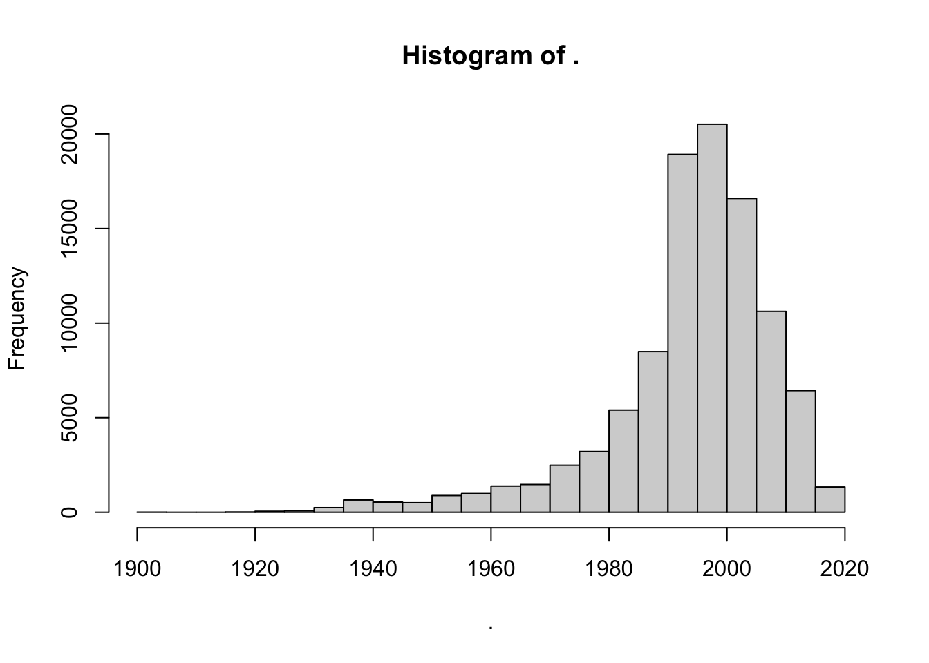
Looks pretty good. Let’s create a new variable called year that contains the year of release of the movie.

movies <- mutate(movies, year = str_extract(title, "[0-9]{4}(?=\\)$)") %>% 
  as.numeric())
summary(movies$year)

##    Min. 1st Qu.  Median    Mean 3rd Qu.    Max.    NA's 
##    1902    1990    1997    1994    2003    2018      30

Whoops. We have 30 NA years. Let’s take a look and see what happened.

movies %>% filter(is.na(year)) %>% 
  select(title)

## # A tibble: 30 x 1
##    title                                                
##    <chr>                                                
##  1 "Black Mirror"                                       
##  2 "Runaway Brain (1995) "                              
##  3 "The Adventures of Sherlock Holmes and Doctor Watson"
##  4 "Maria Bamford: Old Baby"                            
##  5 "Generation Iron 2"                                  
##  6 "Ready Player One"                                   
##  7 "Babylon 5"                                          
##  8 "Ready Player One"                                   
##  9 "Nocturnal Animals"                                  
## 10 "Guilty of Romance (Koi no tsumi) (2011) "           
## # … with 20 more rows

Aha! Some of the movies don’t have years, others have an extra space after the end parentheses. We can handle the extra space with \\s*, which matches zero or more spaces.

pattern = "[0-9]{4}(?=\\)\\s*$)"
movies <- mutate(movies,
  year = str_extract(title, pattern) %>% as.numeric()
)
summary(movies$year)

##    Min. 1st Qu.  Median    Mean 3rd Qu.    Max.    NA's 
##    1902    1990    1997    1994    2003    2018      17

Finally, what were the five highest rated movies of 1999 that had at least 50 ratings?

movies %>% 
  filter(year == 1999) %>% 
  group_by(title) %>% 
  summarize(mean = mean(rating), count = n()) %>% 
  filter(count >= 50) %>% 
  arrange(desc(mean)) %>% 
  print(n = 5)

## # A tibble: 23 x 3
##   title                   mean count
##   <chr>                  <dbl> <int>
## 1 Fight Club (1999)       4.27   218
## 2 Matrix, The (1999)      4.19   278
## 3 Green Mile, The (1999)  4.15   111
## 4 Office Space (1999)     4.09    94
## 5 American Beauty (1999)  4.06   204
## # … with 18 more rows

One final common usage of regular expressions is within select. If your data frame has a lot of variables, and you want to select out some that follow a certain pattern, then knowing regular expressions can be very helpful.

Example 2.9

Consider the accelerometer data in the fosdata package. This data set will be described in more detail in Chapter 8.

accelerometer <- fosdata::accelerometer
names(accelerometer)

##  [1] "participant"                        
##  [2] "machine"                            
##  [3] "set"                                
##  [4] "contraction_mode"                   
##  [5] "time_video_rater_cv_ms"             
##  [6] "time_video_rater_dg_ms"             
##  [7] "time_smartphone_1_ms"               
##  [8] "time_smartphone_2_ms"               
##  [9] "video_rater_mean_ms"                
## [10] "smartphones_mean_ms"                
## [11] "relative_difference"                
## [12] "difference_video_smartphone_ms"     
## [13] "mean_video_smartphone_ms"           
## [14] "contraction_mode_levels"            
## [15] "difference_video_raters_ms"         
## [16] "difference_smartphones_ms"          
## [17] "video_smartphone_difference_outlier"
## [18] "rater_difference_outlier"           
## [19] "smartphone_difference_outlier"      
## [20] "normalized_error_smartphone"        
## [21] "participant_age_levels"             
## [22] "participant_age_years"              
## [23] "participant_height_cm"              
## [24] "participant_weight_kg"              
## [25] "participant_gender"

Look at all of those variables! Most of the data sets that we see in this book have been condensed, but it is not at all uncommon for experimenters to collect data on 30-200 values. Let’s suppose you wanted to create a new data frame that had all of the time measurements in it. Those are the variables whose names end with ms. We can do this by combining select with the regular expression ms$, which matches the letters ms and the end of the string.

select(accelerometer, matches("ms$")) %>% 
  print(n = 5)

## # A tibble: 12,245 x 10
##   time_video_rate… time_video_rate… time_smartphone… time_smartphone…
##              <dbl>            <dbl>            <dbl>            <dbl>
## 1             1340             1360             1650             1700
## 2             1160             1180             1350             1350
## 3             1220             1240             1400             1350
## 4             1260             1280             1400             1350
## 5             1560             1180             1350             1300
## # … with 12,240 more rows, and 6 more variables:
## #   video_rater_mean_ms <dbl>, smartphones_mean_ms <dbl>,
## #   difference_video_smartphone_ms <dbl>,
## #   mean_video_smartphone_ms <dbl>, difference_video_raters_ms <dbl>,
## #   difference_smartphones_ms <dbl>

To build a data frame that includes both variables that start with smartphone or end with ms, use the regular expression | character for “or”.

select(accelerometer, matches("^smartphone|ms$")) %>% 
  print(n = 5)

## # A tibble: 12,245 x 11
##   time_video_rate… time_video_rate… time_smartphone… time_smartphone…
##              <dbl>            <dbl>            <dbl>            <dbl>
## 1             1340             1360             1650             1700
## 2             1160             1180             1350             1350
## 3             1220             1240             1400             1350
## 4             1260             1280             1400             1350
## 5             1560             1180             1350             1300
## # … with 12,240 more rows, and 7 more variables:
## #   video_rater_mean_ms <dbl>, smartphones_mean_ms <dbl>,
## #   difference_video_smartphone_ms <dbl>,
## #   mean_video_smartphone_ms <dbl>, difference_video_raters_ms <dbl>,
## #   difference_smartphones_ms <dbl>,
## #   smartphone_difference_outlier <lgl>

The structure of data

Tidy data: pivoting

The tidyverse is designed for tidy data, and a key feature of tidy data is that all data should be stored in a rectangular array, with each row an observation and each column a variable. In particular, no information should be stored in variable names. As an example, consider the built in data set WorldPhones which gives the number of telephones in each region of the world, back in the day when telephones were still gaining popularity as a device for making phone calls.

The WorldPhones data is stored as a matrix with row names, so we convert it to a tibble called phones and preserve the row names in a new variable called Year. We also clean up the names into a standard format using janitor::clean_names.

phones <- as_tibble(WorldPhones, rownames = "year") %>% 
  janitor::clean_names()
phones

## # A tibble: 7 x 8
##   year  n_amer europe  asia s_amer oceania africa mid_amer
##   <chr>  <dbl>  <dbl> <dbl>  <dbl>   <dbl>  <dbl>    <dbl>
## 1 1951   45939  21574  2876   1815    1646     89      555
## 2 1956   60423  29990  4708   2568    2366   1411      733
## 3 1957   64721  32510  5230   2695    2526   1546      773
## 4 1958   68484  35218  6662   2845    2691   1663      836
## 5 1959   71799  37598  6856   3000    2868   1769      911
## 6 1960   76036  40341  8220   3145    3054   1905     1008
## 7 1961   79831  43173  9053   3338    3224   2005     1076

Notice that the column names are regions of the world, so that there is useful information stored in those names.

Every entry in this data set gives the value for a year and a region, so the tidy format should instead have three variables: year, region, and telephones. Making this change will cause this data set to become much longer. Instead of 7 rows and 7 columns, we will have 49 rows, one for each of the \(7\times7\) year and region combinations. The tool to make this change is the pivot_longer function from the tidyr package (part of the tidyverse):

library(tidyr)
phones %>% 
  pivot_longer(cols = -year, names_to="region", values_to="telephones")

## # A tibble: 49 x 3
##    year  region   telephones
##    <chr> <chr>         <dbl>
##  1 1951  n_amer        45939
##  2 1951  europe        21574
##  3 1951  asia           2876
##  4 1951  s_amer         1815
##  5 1951  oceania        1646
##  6 1951  africa           89
##  7 1951  mid_amer        555
##  8 1956  n_amer        60423
##  9 1956  europe        29990
## 10 1956  asia           4708
## # … with 39 more rows

This function used four arguments. The first was the data frame we wanted to pivot, in this case phones. Second, we specified which columns to use, with the expression cols = -year, which meant “all columns except year”. Finally, we told the function that the names of the columns should become a new variable called “region”, and the values in those columns should become a new variable called “telephones”.

Example 2.10

As a more complex example, let’s look at the billboard data set provided with the tidyr package. This contains the weekly Billboard rankings for each song that entered the top 100 during the year 2000. Observe that each row is a song (track) and the track’s place on the charts is stored in up to 76 columns named wk1 through wk76. There are many NA in the data since none of these tracks were ranked for 76 consecutive weeks.

billboard %>% head(n=5)

## # A tibble: 5 x 79
##   artist track date.entered   wk1   wk2   wk3   wk4   wk5   wk6   wk7
##   <chr>  <chr> <date>       <dbl> <dbl> <dbl> <dbl> <dbl> <dbl> <dbl>
## 1 2 Pac  Baby… 2000-02-26      87    82    72    77    87    94    99
## 2 2Ge+h… The … 2000-09-02      91    87    92    NA    NA    NA    NA
## 3 3 Doo… Kryp… 2000-04-08      81    70    68    67    66    57    54
## 4 3 Doo… Loser 2000-10-21      76    76    72    69    67    65    55
## 5 504 B… Wobb… 2000-04-15      57    34    25    17    17    31    36
## # … with 69 more variables: wk8 <dbl>, wk9 <dbl>, wk10 <dbl>,
## #   wk11 <dbl>, wk12 <dbl>, wk13 <dbl>, wk14 <dbl>, wk15 <dbl>,
## #   wk16 <dbl>, wk17 <dbl>, wk18 <dbl>, wk19 <dbl>, wk20 <dbl>,
## #   wk21 <dbl>, wk22 <dbl>, wk23 <dbl>, wk24 <dbl>, wk25 <dbl>,
## #   wk26 <dbl>, wk27 <dbl>, wk28 <dbl>, wk29 <dbl>, wk30 <dbl>,
## #   wk31 <dbl>, wk32 <dbl>, wk33 <dbl>, wk34 <dbl>, wk35 <dbl>,
## #   wk36 <dbl>, wk37 <dbl>, wk38 <dbl>, wk39 <dbl>, wk40 <dbl>,
## #   wk41 <dbl>, wk42 <dbl>, wk43 <dbl>, wk44 <dbl>, wk45 <dbl>,
## #   wk46 <dbl>, wk47 <dbl>, wk48 <dbl>, wk49 <dbl>, wk50 <dbl>,
## #   wk51 <dbl>, wk52 <dbl>, wk53 <dbl>, wk54 <dbl>, wk55 <dbl>,
## #   wk56 <dbl>, wk57 <dbl>, wk58 <dbl>, wk59 <dbl>, wk60 <dbl>,
## #   wk61 <dbl>, wk62 <dbl>, wk63 <dbl>, wk64 <dbl>, wk65 <dbl>,
## #   wk66 <lgl>, wk67 <lgl>, wk68 <lgl>, wk69 <lgl>, wk70 <lgl>,
## #   wk71 <lgl>, wk72 <lgl>, wk73 <lgl>, wk74 <lgl>, wk75 <lgl>,
## #   wk76 <lgl>

This data is not tidy, since the week column names contain information. To do any sort of analysis on this data, the week needs to be a variable. We use pivot_longer to replace all 76 week columns with two columns, one called “week” and another called “rank”:

long.bill <- billboard %>%
  pivot_longer(cols = wk1:wk76,
               names_to = "week", values_to = "rank",
               values_drop_na = TRUE)
long.bill

## # A tibble: 5,307 x 5
##    artist  track                   date.entered week   rank
##    <chr>   <chr>                   <date>       <chr> <dbl>
##  1 2 Pac   Baby Don't Cry (Keep... 2000-02-26   wk1      87
##  2 2 Pac   Baby Don't Cry (Keep... 2000-02-26   wk2      82
##  3 2 Pac   Baby Don't Cry (Keep... 2000-02-26   wk3      72
##  4 2 Pac   Baby Don't Cry (Keep... 2000-02-26   wk4      77
##  5 2 Pac   Baby Don't Cry (Keep... 2000-02-26   wk5      87
##  6 2 Pac   Baby Don't Cry (Keep... 2000-02-26   wk6      94
##  7 2 Pac   Baby Don't Cry (Keep... 2000-02-26   wk7      99
##  8 2Ge+her The Hardest Part Of ... 2000-09-02   wk1      91
##  9 2Ge+her The Hardest Part Of ... 2000-09-02   wk2      87
## 10 2Ge+her The Hardest Part Of ... 2000-09-02   wk3      92
## # … with 5,297 more rows

The values_drop_na = TRUE argument removes the NA values from the rank column while pivoting.

Which 2000 song spent the most weeks on the charts? This question would have been near impossible to answer without tidying the data. Now we can group by track and count the number of times it was ranked:

long.bill %>%
  group_by(track) %>%
  summarize(weeks_on_chart = n()) %>%
  top_n(n=1, wt=weeks_on_chart)

## # A tibble: 1 x 2
##   track  weeks_on_chart
##   <chr>           <int>
## 1 Higher             57

“Higher”, by Creed, entered the charts in 2000 and spent 57 weeks in the top 100 (though not consecutively!)

The tidyr package also provides a function pivot_wider which performs the opposite transformation to pivot_longer. You will need to provide a names_from value, which contains the variable name to get the column names from, and a values_from value or values, which gives the columns to get the cell values from. You often will also need to provide an id_cols which uniquely identifes each observation. Let’s see how to use it in an example.

::: example {#exm:babynamesfirst} Consider the babynames data set in the babynames package. This consists of all names of babies born in the USA from 1880 through 2017, together with the sex assigned to the baby, the number of babies of that sex given that name in that year, and the proportion of babies with that sex in that year that were given the name. Only names that were given to five or more babies are included.

library(babynames)
head(babynames)

## # A tibble: 6 x 5
##    year sex   name          n   prop
##   <dbl> <chr> <chr>     <int>  <dbl>
## 1  1880 F     Mary       7065 0.0724
## 2  1880 F     Anna       2604 0.0267
## 3  1880 F     Emma       2003 0.0205
## 4  1880 F     Elizabeth  1939 0.0199
## 5  1880 F     Minnie     1746 0.0179
## 6  1880 F     Margaret   1578 0.0162

Convert the babynames data from year 2000 into wide format, where each row is a name together with the number of male babies and female babies with that name. Note that we need to either select down to the variables of interest or we would need to provide the id columns.

babynames %>% 
  filter(year == 2000) %>% 
  pivot_wider(id_cols = name, names_from = sex, values_from = n)

## # A tibble: 27,512 x 3
##    name          F     M
##    <chr>     <int> <int>
##  1 Emily     25953    30
##  2 Hannah    23080    25
##  3 Madison   19967   138
##  4 Ashley    17997    82
##  5 Sarah     17697    26
##  6 Alexis    17629  2714
##  7 Samantha  17266    21
##  8 Jessica   15709    27
##  9 Elizabeth 15094    22
## 10 Taylor    15078  2853
## # … with 27,502 more rows

Not every name had both a male and a female entry. Those are listed as NA in the data frame. If we would prefer them to be 0, we can add values_fill = 0.

Now that we have the data in a nice format, let’s determine the most common name for which the number of male babies was within 200 of the number of female babies.

babynames %>% 
  filter(year == 2000) %>% 
  pivot_wider(id_cols = name, names_from = sex,
              values_from = n, values_fill = 0) %>% 
  filter(M > F - 200, M < F + 200) %>% 
  mutate(total_names = F +  M) %>% 
  top_n(5, total_names)

## # A tibble: 5 x 4
##   name        F     M total_names
##   <chr>   <int> <int>       <int>
## 1 Peyton   1967  2001        3968
## 2 Skyler   1284  1472        2756
## 3 Jessie    719   533        1252
## 4 Sage      557   392         949
## 5 Justice   477   656        1133

We see by this criteria, Peyton is the most common gender neutral name, followed by Skyler, Jessie, Justice and Sage.

You can see another example of how pivot_wider is used in Example ??.

3.10.1 Using join to merge data frames

In this section, we briefly introduce the join family of functions, by focusing on left_join. The function left_join joins two data frames together into one. The syntax is left_join(x, y, by = NULL), where x and y are data frames and by is a list of columns that you want to join the data frames by (there are additional arguments that we won’t be using). The way I remember what left_join does is that it adds the columns of y to the columns of x by matching on columns with the same names.

As an easy example, consider the band_members and band_instruments data sets, both of which are included in the dplyr package.

band_members

## # A tibble: 3 x 2
##   name  band   
##   <chr> <chr>  
## 1 Mick  Stones 
## 2 John  Beatles
## 3 Paul  Beatles

band_instruments

## # A tibble: 3 x 2
##   name  plays 
##   <chr> <chr> 
## 1 John  guitar
## 2 Paul  bass  
## 3 Keith guitar

left_join(band_members, band_instruments)

## Joining, by = "name"

## # A tibble: 3 x 3
##   name  band    plays 
##   <chr> <chr>   <chr> 
## 1 Mick  Stones  <NA>  
## 2 John  Beatles guitar
## 3 Paul  Beatles bass

Now, what happens if Paul learns how to play the drums as well?

band_instruments

## # A tibble: 4 x 2
##   name  plays 
##   <chr> <chr> 
## 1 John  guitar
## 2 Paul  bass  
## 3 Keith guitar
## 4 Paul  drums

left_join(band_members, band_instruments)

## Joining, by = "name"

## # A tibble: 4 x 3
##   name  band    plays 
##   <chr> <chr>   <chr> 
## 1 Mick  Stones  <NA>  
## 2 John  Beatles guitar
## 3 Paul  Beatles bass  
## 4 Paul  Beatles drums

We see that if there are multiple matches to name, then left_join makes multiple rows in the new data frame.

We also used left_join to transform the movies data set that we have been working with throughout this chapter. The original files as downloaded from MovieLens were as follows.

movies <- read.csv("https://stat.slu.edu/~speegle/data/ml-small/movies.csv")
ratings <-
  read.csv("https://stat.slu.edu/~speegle/data/ml-small/ratings.csv")

The movies file contained the movie names and genres, while the ratings file contained the user ID, the rating, and the timestamp.

head(movies)

##   movieId                              title
## 1       1                   Toy Story (1995)
## 2       2                     Jumanji (1995)
## 3       3            Grumpier Old Men (1995)
## 4       4           Waiting to Exhale (1995)
## 5       5 Father of the Bride Part II (1995)
## 6       6                        Heat (1995)
##                                        genres
## 1 Adventure|Animation|Children|Comedy|Fantasy
## 2                  Adventure|Children|Fantasy
## 3                              Comedy|Romance
## 4                        Comedy|Drama|Romance
## 5                                      Comedy
## 6                       Action|Crime|Thriller

head(ratings)

##   userId movieId rating timestamp
## 1      1       1      4 964982703
## 2      1       3      4 964981247
## 3      1       6      4 964982224
## 4      1      47      5 964983815
## 5      1      50      5 964982931
## 6      1      70      3 964982400

We combine the two data sets using left_join to get the one that we used throughout the chapter.

movies <- left_join(movies, ratings, by = "movieId")

Good, now, when would you use this? Well, many times you have data from multiple sources that you want to combine into one data frame.

Example 5.65

Consider the data sets pres_election available in the fosdata package, and unemp available in the mapproj package. These data sets give the by county level presidential election results from 2000-2016, and the population and unemployment rate of all counties in the US. (Note: unemp is from the mapproj package. You may also install that package and use data("unemp")).)

pres_election <- fosdata::pres_election
library(mapproj)

## Loading required package: maps

data("unemp")

Suppose we want to create a new data frame that contains both the election results and the unemployment data. That is a job for left_join.

combined_data <- left_join(pres_election, unemp, by = c("FIPS" = "fips"))

Because the two data frames didn’t have any column names in common, the join required by = to specify which columns to join by.

head(combined_data)

##   year   state state_po  county FIPS    office      candidate
## 1 2000 Alabama       AL Autauga 1001 President        Al Gore
## 2 2000 Alabama       AL Autauga 1001 President George W. Bush
## 3 2000 Alabama       AL Autauga 1001 President    Ralph Nader
## 4 2000 Alabama       AL Autauga 1001 President          Other
## 5 2000 Alabama       AL Baldwin 1003 President        Al Gore
## 6 2000 Alabama       AL Baldwin 1003 President George W. Bush
##        party candidatevotes totalvotes  version   pop unemp
## 1   democrat           4942      17208 20191203 23288   9.7
## 2 republican          11993      17208 20191203 23288   9.7
## 3      green            160      17208 20191203 23288   9.7
## 4         NA            113      17208 20191203 23288   9.7
## 5   democrat          13997      56480 20191203 81706   9.1
## 6 republican          40872      56480 20191203 81706   9.1

Word to the wise: when dealing with spatial data that is organized by county, it is much easier to use the fips code than the county name, because there are variances in capitalization and other issues that come up when trying to use county names.

3.11 The apply family

The focus of this book is on using dplyr tools when manipulating data sets. However, there will be times when it will be useful to know the base R tools for doing some of the same tasks. At a minimum, it can be useful to know these tools when reading other people’s code! The apply family consists of quite a few functions, including apply, sapply, lapply, vapply, tapply, mapply and even replicate! While tapply and its variants might be the closest in spirit to the way we were using dplyr in this chapter, we will focus on apply and sapply.

All of the functions in the apply family are implicit loops, like replicate. The typical usage of apply is apply(X, MARGIN, FUN). The function apply applies the function FUN to either the rows or columns of X, depending on whether MARGIN is 1 (rows) or 2 (columns). So, the argument X is typically a matrix or data frame, MARGIN is either 1 or 2, and FUN is a function, such as sum or mean.

Example 5.66

Consider the data set USJudgeRatings, which contains the ratings of US judges by lawyers on various facets.

head(USJudgeRatings)

##                CONT INTG DMNR DILG CFMG DECI PREP FAMI ORAL WRIT PHYS
## AARONSON,L.H.   5.7  7.9  7.7  7.3  7.1  7.4  7.1  7.1  7.1  7.0  8.3
## ALEXANDER,J.M.  6.8  8.9  8.8  8.5  7.8  8.1  8.0  8.0  7.8  7.9  8.5
## ARMENTANO,A.J.  7.2  8.1  7.8  7.8  7.5  7.6  7.5  7.5  7.3  7.4  7.9
## BERDON,R.I.     6.8  8.8  8.5  8.8  8.3  8.5  8.7  8.7  8.4  8.5  8.8
## BRACKEN,J.J.    7.3  6.4  4.3  6.5  6.0  6.2  5.7  5.7  5.1  5.3  5.5
## BURNS,E.B.      6.2  8.8  8.7  8.5  7.9  8.0  8.1  8.0  8.0  8.0  8.6
##                RTEN
## AARONSON,L.H.   7.8
## ALEXANDER,J.M.  8.7
## ARMENTANO,A.J.  7.8
## BERDON,R.I.     8.7
## BRACKEN,J.J.    4.8
## BURNS,E.B.      8.6

Which judge had the highest mean rating? Which rating scale had the highest mean across all judges?

Using apply across rows computes the mean rating for each judge.

head(apply(USJudgeRatings, MARGIN = 1, mean))

##  AARONSON,L.H. ALEXANDER,J.M. ARMENTANO,A.J.    BERDON,R.I. 
##       7.291667       8.150000       7.616667       8.458333 
##   BRACKEN,J.J.     BURNS,E.B. 
##       5.733333       8.116667

To pull the highest mean rating:

max(apply(USJudgeRatings, MARGIN = 1, mean))

## [1] 8.858333

which.max(apply(USJudgeRatings, MARGIN = 1, mean))

## CALLAHAN,R.J. 
##             7

We see that RJ Callahan had the highest rating of 8.858333.

Using apply across columns computes the mean rating of all of the judges in each category.

apply(USJudgeRatings, MARGIN = 2, mean)

##     CONT     INTG     DMNR     DILG     CFMG     DECI     PREP     FAMI 
## 7.437209 8.020930 7.516279 7.693023 7.479070 7.565116 7.467442 7.488372 
##     ORAL     WRIT     PHYS     RTEN 
## 7.293023 7.383721 7.934884 7.602326

Judges scored highest on the Integrity scale.

The sapply function has as its typical usage sapply(X, FUN), where X is a vector, and FUN is the function that we wish to act on each element of X. Unfortunately, sapply is not type consistent in the way it simplifies results, sometimes returing a vector, sometimes a matrix. This gives sapply a bad reputation, but it is still useful for exploratory analysis.

Example 5.67

Approximate the sd of a \(t\) random variable with 5, 10, 15, 20, 25 and 30 degrees of freedom.

To do this for 5 df, we simulate 10000 random values of \(t\) and take the standard deviation:

sd(rt(10000, df=5))

## [1] 1.274333

To repeat this computation for the other degrees of freedom, turn the simulation into a function and use sapply to feed it each of the df values.

sapply( X = seq(5,30,5), FUN = function(n) sd(rt(10000, df=n)) )

## [1] 1.288595 1.121219 1.080093 1.060021 1.042957 1.032986

sapply took each element of the vector X, applied the function to it, and returned the results as a vector. The symbol n in function(n) is a dummy variable, and can be replaced by any legal R variable name.

The function replicate is a “convenience wrapper” for a common usage of sapply, so that replicate(100, {expr}) is equivalent to sapply(1:100, function(x) {expr}), where in this case, the function inside of sapply will have no dependence on x.

Vignette: dplyr Murder Mystery

The dplyr murder mystery is a whodunnit, where you use your dplyr skillz to analyze data sets that lead to the solution of a murder mystery. The original caper of this sort was the Command Line Murder Mystery, which was recast as SQL Murder Mystery. We have created an R package that is a small modification of the SQL Murder Mystery for you to enjoy. You can download the package via

remotes::install_github(repo = "speegled/dplyrmurdermystery")

Once you install the package, you can load the data into your environment by typing

library(dplyrmurdermystery)
data("dplyr_murder_mystery")

This loads quite a bit of data into your environment, so you may want to make sure you are starting with a clean environment before you do it.

The prompt for this mystery is the following:

There has been a murder in dplyr City! You have lost your notes, but you remember that the murder took place on January 15, 2018 in dplyr City. All of the clues that you will need to solve the murder in contained in the dplyrmurdermystery package, and loaded into you environment.

Vignette: Data and gender

In most studies with human subjects, the investigators collect demographic information on their subjects to control for lurking variables that may interact with the variables under investigation. One of the most commonly collected demographic variables is gender. In this vignette, we discuss current best practices for collecting gender information in surveys and studies.

Why not male or female?

The term transgender refers to people whose gender expression defies social expectations. More narrowly, the term transgender refers to people whose gender identity or gender expression differs from expectations associated with the sex assigned at birth<sup>22</sup>.

Approximately 1 in 250 adults in the U.S. identify as transgender, with that proportion expected to rise as survey questions improve and stigma decreases.<sup>23</sup> For teenagers, this proportion may be as high as 0.7%.<sup>24</sup>

The traditional “Male or Female?” survey question fails to measure the substantial transgender population, and the under- or non-representation of transgender individuals is a barrier to understanding social determinants and health disparities faced by this population.

How to collect gender information

Best practices<sup>25</sup> in collecting gender information are to use a two-step approach, with the following questions:

1. Assigned sex at birth: What sex were you assigned at birth, on your original birth certificate?

• Male
• Female

2. Current gender identity: How do you describe yourself? (check one)

• Male
• Female
• Transgender
• Do not identify as female, male, or transgender

These questions serve as guides. Question 1 has broad agreement, while there is still discussion and research being done as to what the exact wording of Question 2 should be. It is also important to talk to people who have expertise in or familiarity with the specific population you wish to sample from, to see whether there are any adjustments to terminology or questions that should be made for that population.

In general, questions related to sex and gender are considered “sensitive”. Respondents may be reluctant to answer sensitive questions or may answer inaccurately. For these questions, privacy matters. When possible, place sensitive questions on a self-administered survey. Placing gender and sexual orientation questions at the start of a survey may also decrease privacy, since those first questions are encountered at the same time for all subjects and are more visible on paper forms.

How to incorporate gender in data analysis

The relatively small samples of transgender populations create challenges for analysis. One type of error is called a specificity error, and occurs when subjects mistakenly indicate themselves as transgender or another gender minority. The transgender population is less than 1% of the overall population. So, if even one in one hundred subjects misclassify themselves, then the subjects identifying as transgender in the sample will be a mix of half transgender individuals and half misclassified individuals. The best way to combat specificity errors is with carefully worded questions and prepared language to explain the options if asked.

Small samples lead to large margin of error, and make it difficult to detect statistically significant differences within groups. For an individual survey, this may prevent analysis of fine-grained gender information. Aggregating data over time, space, and across surveys can allow analysis of gender minority groups.

Example We should get an example of some data with the two-step gender question.

Exercises

---

Exercises 5.41 - 5.42 require material through Section ??.

5.41

Consider the austen data set in the fosdata package. This data frame contains the complete texts of Emma and Pride and Prejudice, with additional information which you can read about in the help page for the data set.

1. Create a new data frame that consists only of the words in Emma.
2. Create a new data frame that contains only the variables word, word_length and novel.
3. Create a new data frame that has the words in both books arranged in descending word length.
4. Create a new data frame that contains only the longest words that appeared in either of the books.
5. What was the mean word length in the two books together?
6. Create a new data frame that consists only of the distinct words found in the two books, together with the word length and sentiment score variables. This requires you to use both select and distinct.

5.42

Consider the barnacles data set in the fosdata package. This data consists of the counts of the number of barnacles on coral reefs, the area of coral reef that was counted, the perent of coral cover, and the depth of the coral reef. More information can be found in the help page of fosdata::barnacles. Create a new data frame that contains, in addition to the other variables, a variable count_per_m, which is the number of barnacles divided by the area of reef.

---

Exercises 5.43 - 5.65 require material through Section ??.

5.43

Consider the mpg data set in the ggplot2 package.

1. Which car(s) had the highest highway gas mileage? (For the purposes of this question, consider each observation a different car.)
2. Compute the mean city mileage for compact cars.
3. Compute the mean city mileage for each class of cars, and arrange in decreasing order.
4. Which cars have the smallest absolute difference between highway mileage and city mileage? (For the purposes of this question, consider each observation a different “car”.)
5. Compute the mean highway mileage for each year, and arrange in decreasing order.

5.44

This question uses the DrinksWages from the HistData package. This data, gathered by Karl Pearson in 1910, was a survey of people working in various trades (bakers, plumbers, goldbeaters, etc.). The trades are assigned class values of A, B, or C based on required skill. For each trade, he counted the number of workers who drink (drinks), number of sober workers (sober), and recorded wage information (wage). There is also a column n = drinks + sober which is the total number of workers surveyed for each trade.

1. Compute the mean wages for each class, A, B, and C.
2. Find the three trades with the highest proportion of drinkers. Consider only trades with 10 or more workers in the survey.

5.45

Consider the dataset oly12 from the VGAMdata package (that you will probably need to install). It has individual competitor information from the Summer 2012 London Olympic Games.

1. According to this data, which country won the most medals? How many did that country win? (You need to sum Gold, Silver, and Bronze)
2. Which countries were the heaviest? Compute the mean weight of male athletes for all countries with at least 10 competitors, and report the top three.

---

Exercises 5.46 - 5.50 all use the movies data set from the fosdata library.

5.46

What is the movie with the highest mean rating that has been rated at least 30 times?

5.47

Which genre has been rated the most? (For the purpose of this, consider Comedy and Comedy|Romance completely different genres, for example.)

5.48

Which movie in the genre Comedy|Romance that has been rated at least 50 times has the lowest mean rating? Which has the highest mean rating?

5.49

Which movie that has a mean rating of 4 or higher has been rated the most times?

5.50

Which user gave the highest mean ratings?

---

Exercises 5.51 - 5.56 all use the Batting data set from the Lahman library. This gives the batting statistics of every player who has played baseball from 1871 through the present day.

5.51

Which player has been hit-by-pitch the most number of times?

5.52

How many doubles were hit in 1871?

5.53

Which team has the most total number of home runs, all time?

5.54

Which player who has played in at least 500 games has scored the most number of runs per game?

5.55

1. Which player has the most lifetime at bats without ever having hit a home run?
2. Which active player has the most lifetime at bats without ever having hit a home run? (An active player is someone with an entry in the most recent year of the data set).

5.56

Make sure to take into account stint in these problems.

1. Verify that Curtis Granderson hit the most triples in a single season since 1960.
2. In which season did the major league leader in triples have the fewest triples?
3. In which season was there the biggest difference between the major league leader in stolen bases (SB) and the player with the second most stolen bases?

---

Exercises 5.57 - 5.64 all use the Pitching data set from the Lahman library. This gives the pitching statistics of every pitcher who has played baseball from 1871 through the present day.

5.57

1. Which pitcher has won (W) the most number of games?
2. Which pitcher has lost (L) the most number of games?

5.58

Which pitcher has hit the most opponents with a pitch (HBP)?

5.59

Which year had the most number of complete games (CG)?

5.60

Among pitchers who have won at least 100 games, which has the highest winning percentage? (Winning percentage is wins divided by wins + losses.)

5.61

Among pitchers who have struck out at least 500 batters, which has the highest strikeout to walk ratio? (Strikeout to walk ratio is SO/BB.)

5.62

List the pitchers for the St Louis Cardinals (SLN) in 2006 with at least 30 recorded outs (IPouts), sorted by ERA from lowest to highest.

5.63

A balk (BK) is a subtle technical mistake that a pitcher can make when throwing. What were the top five years with the most balks in major league baseball history? Why was 1988 known as “the year of the balk”?

5.64

Which pitcher has the most outs pitched (IPouts) of all the pitchers who have more bases on balls (BB) than hits allowed (H)? Who has the second most?

5.65

M&M’s are small pieces of candy that come in various colors and are sold in various sizes of bags. One popular size for Halloween is the “Fun Size,” which typically contains between 15 and 18 M&M’s. For the purposes of this problem, we assume the mean number of candies in a bag is 17 and the standard deviation is 1. According to Rick Wicklin<sup>26</sup>, the proportion of M&M’s of various colors produced in the New Jersey M&M factory are as follows.

Color	Proportion
Blue	25.0
Orange	25.0
Green	12.5
Yellow	12.5
Red	12.5
Brown	12.5

Suppose that you purchase a big bag containing 200 Fun Size M&M packages. The purpose of this exercise it to estimate the probability that each of your bags has a different distribution of colors.

1. We will model the number of M&M’s in a bag with a binomial random variable. Find values of \(n\) and \(p\) such that a binomial random variable with parameters \(n\) and \(p\) has mean approximately 17 and variance approximately 1.
2. (Hard) Create a data frame that has its rows being bags and columns being colors, where each entry is the number of M&M’s in that bag of that color. For example, the first entry in the first column might be 2, the number of Blue M&M’s in the first bag.
3. Use nrows and dplyr::distinct to determine whether each row in the data frame that you created is distinct.
4. Put inside replicate and estimate the probability that all bags will be distinct. This could take some time to run, depending on how you did parts b and c, so start with 500 replicates.

---

Exercises 5.66 - 5.72 require material through Section ??.

5.66

The data set words is built in to the stringr package.

1. How many words in this data set contain “ff”
2. What percentage of these words start with “s”?

5.67

The data set sentences is built in to the stringr package.

1. What percentage of sentences contain the string “the”?
2. What percentage of sentences contain the word “the” (so, either “the” or “The”)?
3. What percentage of sentences start with the word “The”?
4. Find the one sentence that has both an “x” and a “q” in it.
5. Which words are the most common words that a sentence ends with?

5.68

The data set fruit is built in to the stringr package.

1. How many fruits have the word “berry” in their name?
2. Some of these fruit have the word “fruit” in their name. Find these fruit and remove the word “fruit” to create a list of words that can be made into fruit. (Hint: use str_remove)

---

Exercises 5.69 - 5.71 require the babynames data frame from the babynames package.

5.69

Say that a name is popular if it was given to 1000 or more babies of a single sex. How many popular female names were there in 2015? What percentage of these popular female names ended in the letter ‘a’?

5.70

Consider the babynames data set. Restrict to babies born in 2003. We’ll consider a name to be gender neutral if the number of male babies given that name is within plus or minus 20 percent of the number of girl babies given that name. What were the 5 most popular gender neutral names in 2003?

5.71

The phonics package has a function metaphone that gives a rough phonetic transcription of English words. Restrict to babies born in 2003, and create a new variable called phonetic, which gives the phonetic transcription of the names.

1. Filter the data set so that the year is 2003 and so that each phonetic transcription has at least two distinct names associated with it.
2. Filter the data so that it only contains the top 2 most given names for each phonetic transcription.
3. Among the pairs of names for girls obtained in the previous part with the same metaphone representation and such that each name occurs less than 120 percent of the times that the other name occurs, which pair of names was given most frequently?
4. We wouldn’t consider the most common pair to actually be the “same name.” Look through the list sorted by total number of times the pair of names occurs, and state which pair of names that you would consider to be the same name is the most common. That pair is, in some sense, the hardest to spell common name from 2003.
5. What is the most common hard to spell triple of girls names from 2003? (Answers may vary, depending on how you interpret this. To get interesting answers, you may need to loosen the 120 percent rule from the previous part.)

---

5.72

In this exercise, we examine the expected number of tosses until various patterns occur. For each pattern given below, find the expected number of tosses until the pattern occurs. For example, if the pattern is HTH and you toss HHTTHTTHTH, then it would be 10 tosses until HTH occurs. With the same sequence of tosses, it would be 5 tosses until TTH occurs. (Hint: paste(coins, collapse = "") converts a vector containing H and T into a character string on which you can use the stringr commands such as str_locate.)

1. What is the expected number of tosses until HTH occurs?
2. Until HHT occurs?
3. Until TTTT occurs?
4. Until THHH occurs?

---

Exercises 5.73 - 5.74 require material through Section ??.

5.73

This exercise uses the billboard data from the tidyr package.

1. Which artist had the most tracks on the charts in 2000?
2. Which track from 2000 spent the most weeks at #1? (This requires tidying the data as described in section ??)

5.74

Consider the scotland_births data set in the fosdata package. This data gives the number of births by the age of the mother in Scotland for each year from 1945-2019. This data is in wide format. (Completion of this exercise will be helpful for Exercise 6.26.)

1. Convert the data into long format with three variable names: age, year and number, where each observation is the number of babies born in year to mothers that are age years old.
2. Convert the year to integer by removing the x and using as.integer.
3. Which year had the most babies born to mothers 20 years old or younger?

---

Exercises 5.75 - 5.76 require material through Section 3.11.

5.75

Suppose you sample five numbers from a uniform distribution on the interval \([0, 1]\). Use simulation to show that the expected value of the \(k\)th smallest of the five values is \(\frac{k}{6}\). That is, the minimum of the 5 values has expected value 1/6, the second smallest of the values has expected value 2/6, and so on.

5.76

---

8. In this text, we only consider discrete rv’s with integer values, but more generally a discrete rv could take values in any subset of \(\mathbb{R}\) consisting of countably many points.↩︎

9. Gaillard, Jean‐Michel, et al. “One size fits all: Eurasian lynx females share a common optimal litter size.” Journal of Animal Ecology 83.1 (2014): 107-115.↩︎

10. Amos Tversky & Thomas Gilovich (1989) The Cold Facts about the “Hot Hand” in Basketball, CHANCE, 2:1, 16-21↩︎

11. That is, the variance is greater than or equal to zero.↩︎

12. Yihui Xie, J.J. Allaire, Garrett Grolemund, R Markdown The Definitive Guide, Published July 17, 2018 by Chapman and Hall/CRC 304 Pages.↩︎

13. Cunningham, P.W. “The Health 202: The Trump administration is eyeing a new testing strategy for coronavirus, Anthony Fauci says”, Washington Post, June 26, 2020.↩︎

14. Miller, Joshua B. and Sanjurjo, Adam, A Cold Shower for the Hot Hand Fallacy: Robust Evidence that Belief in the Hot Hand is Justified (August 24, 2019). IGIER Working Paper No. 518, Available at SSRN: https://ssrn.com/abstract=2450479 or http://dx.doi.org/10.2139/ssrn.2450479

    :::↩︎

15. Athos EA, Levinson B, Kistler A, et al. Dichotomy and perceptual distortions in absolute pitch ability. Proc Natl Acad Sci U S A. 2007;104(37):14795-14800. doi:10.1073/pnas.0703868104 https://www.ncbi.nlm.nih.gov/pmc/articles/PMC1959403/

    :::↩︎

16. The R function proportions is new to R 4.0.1 and is recommended as a drop-in replacement for the unfortunately named prop.table. Similarly, marginSums is recommended as a drop-in replacement for margin.table.↩︎

17. If you are typing up your work in an .Rmd file, then the plots will not appear on the same graph when executing your code inline, but will they will overlay when you knit your document.↩︎

18. Wackerly, D. D., Mendenhall, W., & Scheaffer, R. L. (2008). Mathematical statistics with applications. Belmont, CA: Thomson Brooks/Cole.↩︎

19. Loading dplyr produces warning messages because the dplyr package contains commands that override some base R commands (notably the filter command). This book will not show these warnings. Use suppressMessages(library(dplyr)) if you want to load the package quietly.↩︎

20. F. Maxwell Harper and Joseph A. Konstan. 2015. The MovieLens Datasets: History and Context. ACM Transactions on Interactive Intelligent Systems (TiiS) 5, 4: 19:1–19:19. https://doi.org/10.1145/2827872↩︎

21. Rating should almost certainly have been reclassified as an ordered factor, and it is not clear that taking the mean is really a valid thing to do.↩︎

22. Berg-Weger, Marla (2016). Social Work and Social Welfare: An Invitation. Routledge. p. 229. ISBN 978-1317592020.↩︎

23. Meerwijk EL, Sevelius JM. Transgender Population Size in the United States: a Meta-Regression of Population-Based Probability Samples. Am J Public Health. 2017;107(2):e1-e8. doi:10.2105/AJPH.2016.303578↩︎

24. Chokshi, N., “One in Every 137 Teenagers Would Identify as Transgender, Report Says”. New York Times, Feb. 23, 2017.↩︎

25. The GenIUSS Group. (2014). Best practices for asking questions to identify transgender and other gender minority respondents on population-based surveys. J.L. Herman (ed.). Los Angeles, CA: the Williams Institute.↩︎

26. Purtill, C. “A statistician got curious about M&M colors and went on an endearingly geeky quest for answers”, Quartz, March 15, 2017. https://qz.com/918008/the-color-distribution-of-mms-as-determined-by-a-phd-in-statistics/↩︎