Chapter 8 Inference on the Mean

Consider the brake data set,⁵⁰ which is available in the fosdata package. The authors noted that there have been several accidents involving unintended acceleration, where the driver was unable to realize that the car was accelerating in time to apply the brakes. This type of accident seems to happen more with older drivers, and the authors developed an experiment to test whether older drivers are less adept at correcting unintended acceleration.

The set-up of the experiment was as follows. Older (65+) drivers and younger (18-32) drivers were recruited. The drivers were put in a simulation, and told to apply the brake when a light turned red. Ninety percent of the time, this would work as desired, but 10 percent of the time, the brake would instead speed up the car.

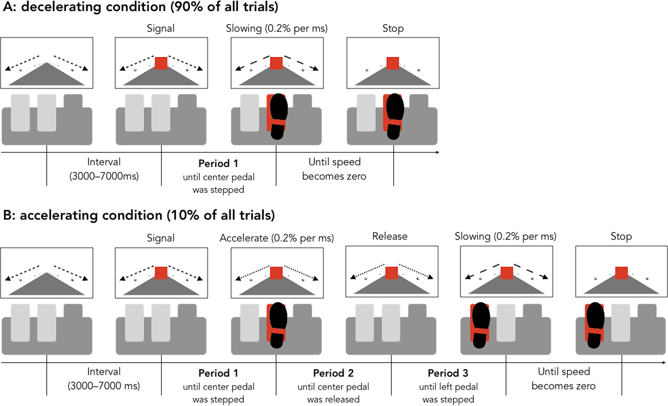
Figure 8.1

Figure 8.1: Figure from Hasegawa, et al

The experimenters measured three things in the 10 percent case.

The length of time before the initial application of the brake.
The length of time before the brake was released.
The length of time before the pedal to the left of the brake was pressed, which would then stop the car.

The experimenters desire was to see whether there is a difference in the true mean times of participants in the different age groups to perform one of the three tasks.

You can get the data via

brake <- fosdata::brake

The authors collected a lot more data than we will be using in this chapter! Let’s look at boxplots of the latency (length of time) in stepping on the pedal after seeing the first red light. The time to step on the pedal after seeing a red light is latency_p1, the time between stepping on the brake and releasing it after realizing that the car is accelerating is latency_p2, and the time to step on the correct pedal after releasing the incorrect pedal is latency_p3.

select(brake, matches("latency_p[1-3]$|age_group")) %>%
  tidyr::pivot_longer(
    cols = starts_with("lat"),
    names_to = "type", values_to = "time"
  ) %>%
  ggplot(aes(x = type, y = time, color = age_group)) +
  geom_boxplot()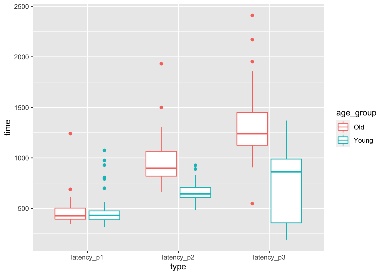

At a first glance, it seems like there may not be a difference in mean time to react to the red light between old and young, but there may well be a difference in the time to realize a mistake has been made. The purpose of this chapter is to be able to systematically study experiments such as this. In Example 8.19, we will be able to test whether the mean length of time for an older driver to release the pedal after it resulted in an unintended acceleration is the same as the mean length of time for a younger driver. We first develop some theory.

8.1 Sampling distribution of the sample mean

In Section 5.5 we discussed various sampling distrubutions for statistics related to a random sample from a population. The $t$ random variable first described in Section 5.5.3 will play an essential role in this chapter, so we review and expand upon that discussion here. Theorem 5.7 states that if $X_1,\ldots,X_n$ are iid normal rv’s with mean $\mu$ and standard deviation $\sigma$, then \[ \frac{\overline{X} - \mu}{S/\sqrt{n}} \sim t_{n-1} \] where $S$ is the sample standard deviation,⁵¹ $\overline{X}$ is the sample mean, and $t_{n-1}$ is a $t$ random variable with $n- 1$ degrees of freedom.

Tryit 8.1

Simulate the pdf of $\frac{\overline{X} - \mu}{S/\sqrt{n}}$ when $n = 3$, $\mu = 5$ and $\sigma = 1$, and compare to the pdf of a $t$ random variable with 2 degrees of freedom.

The following plot compares the pdf of $t$ random variables with various degrees of freedom.

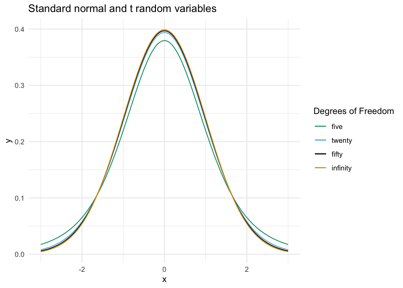
We see that as the number of degrees of freedom increases, the tails of the $t$ distribution become lighter. From the point of view of the sampling distribution of $\frac{\overline{X} - \mu}{S/\sqrt{n}}$, this can be explained through the decrease in uncertainty of the estimate of $\sigma$ by $S$. When we only have 6 samples (so that we have 5 degrees of freedom), we are unsure about our approximation of $\sigma$ by $S$, so the distribution will be more spread out. As the sample size goes to $\infty$, we become more and more sure of our estimate of $\sigma$, until in the limit the $t$ distribution is standard normal.

Theorem 8.1

For $n = 1, 2, \ldots$ let $X_n$ be a $t$ random variable with $n$ degrees of freedom. Let $Z$ be a standard normal random variable. Then, \[ \lim_{n \to \infty} X_n = Z \] in the sense that for every $a < b$, \[ \lim_{n \to \infty} P(a < X_n < b) = P(a < Z < b) \]

The difference between the pdfs of a $t$ random variable and a normal random variable may not appear large in the picture, but it can make a substantial difference in the computation of tail probabilities, which is what we are going to be interested in later in this chapter. If we compare

pt(-2.5, df = 3) - pnorm(-2.5)

## [1] 0.03764366

pt(-2.5, df = 3) / pnorm(-2.5)

## [1] 7.062107

we see that, while the absolute difference in areas is only 0.038, the area under the $t$ curve is about 7 times as large as the corresponding area under the standard normal curve, which is quite a difference. As the degrees of freedom gets larger, however, the difference between these tail probabilities becomes negligible in computations.

We also see from the graphs of the pdfs that $t$ random variables are symmetric about 0, and the likelihood of $x$ decreases as the absolute value of $x$ increases. For example, 0 is the most likely outcome of a $t$ random variable, and the interval $[-1, 1]$ is the most likely interval of length 2.

The remainder of this section is devoted to a computation that illustrates the use of $t$ random variables and their relation to sampling distributions. Suppose that we know neither $\mu$ nor $\sigma$, but we do know that our data is randomly sampled from a normal distribution. Let $t_{\alpha}$ be the unique real number such that $P(t > t_{\alpha}) = \alpha$, where $t$ has $n-1$ degrees of freedom. Note that $t_{\alpha}$ depends on $n$, because the $t$ distribution has more area in its tails when $n$ is small.

Then, we know that \[ P\left( t_{1 - \alpha/2} < \frac{\overline{X} - \mu}{S/\sqrt{n}} < t_{\alpha/2}\right) = 1 - \alpha. \]

By rearranging, we get

\[ P\left(\overline{X} + t_{1 - \alpha/2} S/\sqrt{n} < \mu < \overline{X} + t_{\alpha/2} S/\sqrt{n}\right) = 1 - \alpha. \]

Because the $t$ distribution is symmetric, $t_{1-\alpha/2} = -t_{\alpha/2}$, so we can rewrite the equation symmetrically as:

\[ P\left(\overline{X} - t_{\alpha/2} S/\sqrt{n} < \mu < \overline{X} + t_{\alpha/2} S/\sqrt{n}\right) = 1 - \alpha. \]

Let’s think about what this means. Take $n = 10$ and $\alpha = 0.10$ just to be specific. This means that if we were to repeatedly take 10 samples from a normal distribution with mean $\mu$ and any $\sigma$, then 90% of the time, $\mu$ would lie between $\overline{X} + t_{\alpha/2} S/\sqrt{n}$ and $\overline{X} - t_{\alpha/2} S/\sqrt{n}$. That sounds like something that we need to double check using a simulation!

t05 <- qt(.05, 9, lower.tail = FALSE)
mean(replicate(10000, {
  dat <- rnorm(10, 5, 8) # Choose mean 5 and sd 8
  xbar <- mean(dat)
  SE <- sd(dat) / sqrt(10)
  (xbar - t05 * SE < 5) & (xbar + t05 * SE > 5)
}))

## [1] 0.9002

The first line computes $t_{\alpha/2}$ using qt, the quantile function for the $t$ distribution, here with 9 degrees of freedom. Then we check the inequality given above. It works; the 90 percent confidence interval contains the true mean about 90 percent of the time.

Tryit 8.2

Repeat the above simulation with $n = 20$, $\mu = 7$ and $\alpha = .05$.

8.2 Confidence intervals for the mean

In the previous section, we saw that if $X_1, \ldots, X_n$ is a random sample from a normal population with mean $\mu$, then \[ P\left(\overline{X} - t_{\alpha/2} S/\sqrt{n} < \mu < \overline{X} + t_{\alpha/2} S/\sqrt{n}\right) = 1 - \alpha. \] This leads naturally to the following definition.

Definition 8.1

Given a sample of size $n$ from iid normal random variables, the interval

\[ \left[ \overline{X} - t_{\alpha/2} S/\sqrt{n},\ \ \overline{X} + t_{\alpha/2} S/\sqrt{n} \right] \]

is a 100(1 - $\alpha$)% confidence interval for $\mu$.

“Confidence” means that as the experiment (choosing a sample) is repeated, in the limit the mean $\mu$ will lie in the confidence interval 100(1 - $\alpha$)% of the time.

Example 8.2

Consider the heart rate and body temperature data normtemp.⁵²

You can read normtemp as follows.

normtemp <- fosdata::normtemp

What kind of data is this?

str(normtemp)

## 'data.frame':    130 obs. of  3 variables:
##  $ temp  : num  96.3 96.7 96.9 97 97.1 97.1 97.1 97.2 97.3 97.4 ...
##  $ gender: int  1 1 1 1 1 1 1 1 1 1 ...
##  $ bpm   : int  70 71 74 80 73 75 82 64 69 70 ...

head(normtemp)

##   temp gender bpm
## 1 96.3      1  70
## 2 96.7      1  71
## 3 96.9      1  74
## 4 97.0      1  80
## 5 97.1      1  73
## 6 97.1      1  75

We see that the data set is 130 observations of body temperature and heart rate. There is also gender information attached, that we will ignore for the purposes of this example.

Let’s visualize the data through a boxplot.

ggplot(normtemp, aes(x = " ", y = temp)) +
  geom_boxplot(notch = TRUE)

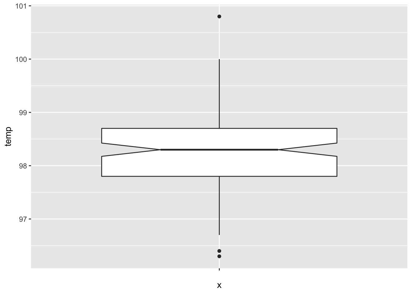
The data looks symmetric without severe outliers, and according to the plot, the true median should be about between 98.2 and 98.4.

Let’s find a 98% confidence interval for the mean body temperature of healthy adults. In order for this to be valid, we are assuming that we have a random sample from all healthy adults (highly unlikely to be formally true), and that the body temperature of healthy adults is normally distributed (also unlikely to be formally true). Later, we will discuss deviations from our assumptions and when we should be concerned.

Using definition 8.1, we have

xbar <- mean(normtemp$temp)
s <- sd(normtemp$temp)
lower_ci <- xbar - s / sqrt(130) * qt(.99, df = 129)
upper_ci <- xbar + s / sqrt(130) * qt(.99, df = 129)

lower_ci

## [1] 98.09776

upper_ci

## [1] 98.40071

The 98 percent confidence interval is $[98.1, 98.4]$. The R command that finds a confidence interval for the mean in one easy step is t.test .

t.test(normtemp$temp, conf.level = .98)

## 
##  One Sample t-test
## 
## data:  normtemp$temp
## t = 1527.9, df = 129, p-value < 2.2e-16
## alternative hypothesis: true mean is not equal to 0
## 98 percent confidence interval:
##  98.09776 98.40071
## sample estimates:
## mean of x 
##  98.24923

We get a lot of information that we will discuss in more detail later. But we see that the confidence interval computed this way agrees with the values we computed above. We are 98 percent confident that the mean body temperature of healthy adults is between 98.1 and 98.4.

Alert 8.1

We are not saying anything about the mean body temperature of the people in the study. That is exactly 98.24923, and we don’t need to do anything fancy. We are making an inference about the mean body temperature of all healthy adults.
Note that to be more precise, we might want to say it is the mean body temperature of all healthy adults as would be measured by this experimenter. Other experimenters could have a different technique for measuring body temperatures which could lead to a different answer.

Alert 8.2

Once we have done the experiment and have a particular interval, it doesn’t make sense to talk about the probability that $\mu$ (a constant) is in the (constant) interval. There is nothing random remaining, and either $\mu$ is in the interval or it is not. Since $\mu$ is typically an unknown value, it is typically impossible to know if the specific confidence interval produced actually does contain $\mu$.

Assumptions 8.1 (For producing a confidence interval)

the population is normal, or the sample size is large enough for the Central Limit Theorem to reasonably apply.
the sample values are independent.

There are several ways that a sample can be dependent, and it is not normally possible to explicitly test whether the sample is independent. Here are a few things to look out for. First, if there is a time component to the data, you should be wary that the samples might depend on time. For example, if the data you are collecting is outdoor temperature, then the temperature observed very well could depend on time. Second, if you are repeating measurements, then the data is not independent. For example, if you have ratings of movies, then it is likely that each person has their own distribution of ratings that they give. So, if you have 10 ratings from each of 5 people, you would not expect the 50 samples to be independent. Third, if there is a change in the experimental setup, then you should not assume independence. We will see an example below where the experimenter changed the experiment after the 6th measurement. We can not assume that the measurements are independent of which setup was used.

To test normality of the population, we will examine histograms and boxplots of the data, calculate skewness, and run simulations to determine how large of a sample size is necessary for the Central Limit Theorem to make up for departures from normality.

We systematically study the robustness to departures from the assumptions in Section 8.5 using simulations.

Now that we have seen confidence intervals for the mean when sampling from a normal distribution, we present the general definition of a confidence interval.

Definition 8.3

Suppose that $X_1, \ldots, X_n$ is a random sample from a population with a parameter $\rho$. A 100(1 - $\alpha$)% confidence interval for a parameter $\rho$ is an interval $[L, U]$, where $L$ and $U$ are functions of $X_1, \ldots, X_n$, such that the probability that $\rho \in [L, U]$ is 100(1 - $\alpha$) for each value of $\rho$.

With this more general definition of confidence interval, we see that there is also a more subtle issue with thinking of confidence as a probability; a procedure which will contain the true parameter value 95% of the time does not necessarily always create intervals that are about 95% “likely” (whatever meaning you attach to that) to contain the parameter value. As an extreme example, consider the following procedure for estimating the mean. It ignores the data and 95% of the time says that the mean is between $-\infty$ and $\infty$. The rest of the time it says the mean is exactly $\pi$. This absurd procedure will contain the true parameter 95% of the time, but the intervals obtained are either 100% or 0% likely to contain the true mean, and when we see which interval we have, we know what the true likelihood is of it containing the mean. Nonetheless, it is widely accepted to say that we are 100(1 - $\alpha$)% confident that the mean is in the interval, which is what we will also do.

8.3 Hypothesis tests of the mean

In this section, we develop the terminology for hypothesis testing of the mean with a single example that runs throughout.

Carl Wunderlich⁵³ claimed to have “got together a material which comprises many thousand complete cases of thermometric observations of disease, and millions of separate readings of temperature.” Based on the measurements he made, he claimed that the mean temperature of healthy adults is 37 degrees Celsius, or 98.6 degrees Fahrenheit. The value of 98.6 degrees for the body temperature of a healthy adult is still widely used.

Now suppose that we wish to revisit the findings of Wunderlich. Perhaps measuring devices have become more accurate in the last 150 years, or perhaps the mean body temperature of healthy adults has changed for some other reason. We wish to test whether the true mean body temperature of healthy adults is 98.6 degrees or whether it is not. This is an example of a hypothesis test.

In hypothesis testing, there is a null hypothesis and an alternative hypothesis. Both null and alternative hypotheses are statements about the population distribution. In the example of mean body temperature, the null hypothesis would be $H_0: \mu = 98.6$ and the alternative hypothesis would be $H_a: \mu \not= 98.6$, where $\mu$ is the true mean body temperature of healthy adults.

Typically, the null hypothesis is the default assumption, or the conventional wisdom about a population. Often it is exactly the thing that a researcher is trying to show is false. The alternative hypothesis states that the null hypothesis is false, sometimes in a particular way.

The purpose of hypothesis testing is to either reject or fail to reject the null hypothesis. A researcher would collect data relating to the population being studied and use a hypothesis test to determine whether the evidence against the null hypothesis (if any) is strong enough to reject the null hypothesis in favor of the alternative hypothesis. In terms of body temperature, we might collect 130 body temperatures of healthy adults. If the mean body temperature of the sample is far enough away from 98.6 relative to the standard deviation of the sample, then that would be sufficient evidence to reject the null hypothesis. Of course, we still need to quantify far enough away in the previous sentence, and it will also depend on the sample size.

For a hypothesis test of the mean, we will construct a test statistic \[ T = \frac{\overline{X} - \mu_0}{S/\sqrt{n}} \] where $\mu_0$ is the value of the mean under the null hypothesis.

Definition 8.4

The rejection region of a hypothesis test is the set of possible values of the test statistic which will lead to a rejection of the null hypothesis.

The $\alpha$ level of a hypothesis test is the probability that a test statistic will have a value in the rejection region given that the null hypothesis is true.

Example 8.5

Suppose in the body temperature example, we have a rejection region of $|T| > 2$. The $\alpha$ level of the test is the probability that $|T| > 2$ when $\mu = 98.6$. Note that when $\mu = 98.6, \, T \sim t_{129}$, so we can compute $\alpha$ via

pt(-2, 129) + pt(2, 129, lower.tail = FALSE)

## [1] 0.04760043

The level of the test in this example would be $\alpha = .0476$.

In practice, we construct the rejection region to have a pre-specified level $\alpha$.

Definition 8.6

In a one-sample hypothesis test of the mean at the level $\alpha$, the rejection region is $|T| > t_{\alpha/2}$, where $t_{\alpha/2} =$ qt(alpha/2, n - 1, lower.tail = FALSE) is the unique value such that $P(t_{n - 1} > t_{\alpha/2}) = \alpha/2$.

Example 8.7

Consider again the temp variable in the normtemp data set in the fosdata package. To construct a rejection region for a hypothesis test at the $\alpha = .02$ level, we compute

qt(.02 / 2, 130 - 1, lower.tail = FALSE)

## [1] 2.355602

So, our rejection region is $|T| > 2.355602$. Our actual value of $|T|$ in this examle is

abs((mean(normtemp$temp) - 98.6) / (sd(normtemp$temp) / sqrt(130)))

## [1] 5.454823

Since this is in the rejection region, we would reject the null hypothesis at the $\alpha = .02$ level that the true mean body temperature of healthy adults is 98.6 degrees Fahrenheit.

Note that in the previous example, the observed value of the test statistic was considerably larger than the smallest value for which we would have rejected the null hypothesis. Indeed, consider the following table of rejection regions corresponding to various levels $\alpha$.

Table 8.1: Rejection Regions when n = 130
alpha	Rejection region \|T\| >
0.01	2.614479
0.001	3.367546
0.0001	4.015720
0.00001	4.599057
0.000001	5.138220
0.0000001	5.645460

We see that we would have rejected the null hypothesis for $\alpha = 0.000001$ but not when $\alpha = 0.0000001.$ The smallest value of $\alpha$ for which we would still reject $H_0$ is called the $p$-value associated with the hypothesis test.

Definition 8.8

Let $X_1, \ldots, X_n$ be a random sample from a normal population with unknown mean $\mu$ and standard deviation. When testing $H_0: \mu = \mu_0$ versus $H_a: \mu \not= \mu_0$, the $p$-value associated with the test is $2 * P(t_{n - 1} > |T|)$, where $t_{n-1}$ is a $t$ random variable with $n - 1$ degrees of freedom and $T = \frac{\overline{X} - \mu_0}{S/\sqrt{n}}$ is the test statistic. The $p$-value is also the smallest level $\alpha$ for which we would reject $H_0$.

Alert 8.3

When conducting a hypothesis test at the level $\alpha$, if the $p$-value is less than $\alpha$ then we reject $H_0$. If the $p$-value is greater than $\alpha$, then we fail to reject $H_0$.

Definition 8.9

In a hypothesis test, if $p < \alpha$, we say the results are statistically significant.

Throughout scientific literature, the term “significance” is used to mean that $H_0$ was rejected by an experiment resulting in a $p$-value less than $\alpha$. More often than not, the value of $\alpha$ is unstated, and implicitly $\alpha = 0.05$ so that “significant” means that $p < 0.05$.

Example 8.10

Continuing with the normtemp data from above, we can compute the $p$-value using R in multiple ways. First, we recall that under the assumption that the underlying population is normal, $T$ has a $t$ distribution with 129 degrees of freedom. The test statistic in our case satisfies $|T| = 5.454823$. The smallest rejection region which would still lead to rejecting $H_0$ is $|T| \ge 5.454823$, which has probability given by

pt(-5.454823, df = 129) + pt(5.454823, df = 129, lower.tail = F)

## [1] 2.410635e-07

This is the $p$-value associated with the test.

As one would expect, R also has automated this procedure in the function t.test. In this case, one would use

t.test(normtemp$temp, mu = 98.6)

## 
##  One Sample t-test
## 
## data:  normtemp$temp
## t = -5.4548, df = 129, p-value = 2.411e-07
## alternative hypothesis: true mean is not equal to 98.6
## 95 percent confidence interval:
##  98.12200 98.37646
## sample estimates:
## mean of x 
##  98.24923

Either way, we get a $p$-value of about 0.000002, which is the probability of obtaining data at least this compelling against $H_0$ when $H_0$ is true. In other words, it is very unlikely that data with a test statistic as large as 5.45 would be collected if the true mean temp of healthy adults is 98.6. (Again, we are assuming a random sample of healthy adults and normal distribution of temperatures of healthy adults.)

Example 8.11

Let’s consider the Cavendish data set in the HistData package. Henry Cavendish carried out experiments in 1798 to determine the mean density of the earth. He collected 29 measurements, but changed the exact set-up of his experiment after the 6th measurement.

The current accepted value for the mean density of the earth is $5.515 \, kg/m^3$. Let’s examine Cavendish’s data from that modern perspective and test $H_0: \mu = 5.515$ versus $H_a: \mu\not= 5.515$. The null hypothesis is that Cavendish’s experimental measurements were unbiased, and that the true mean was the correct value. The alternative is that his set-up had some inherent bias.

A first question that comes up is: what are we going to do with the first six observations? Since the experimental setup was changed after the 6th measurement, it seems likely that the first six observations are not independent of the rest of the observations. Hence, we will proceed by throwing out the first six observations. The variable density3 contains the measurements with the first 6 values removed.

Let’s look at a boxplot of the data.

cavendish <- HistData::Cavendish
ggplot(cavendish, aes(x = "", y = density3)) +
  geom_boxplot(outlier.size = -1) +
  geom_jitter(height = 0, width = 0.2)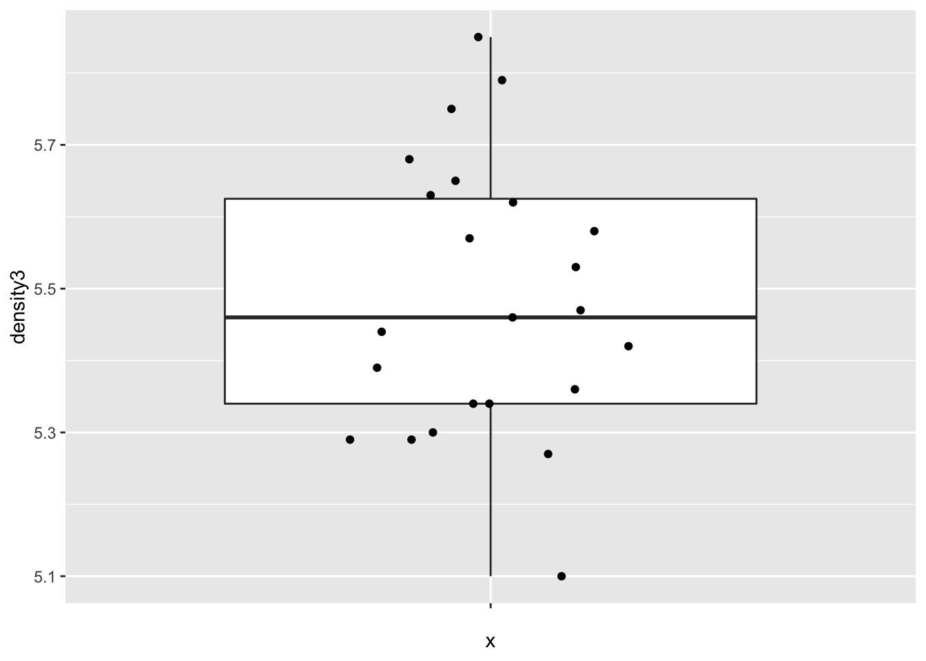

The data appears plausibly to be from a normal distribution, and there are no apparent outliers.

t.test(cavendish$density3, mu = 5.5155)

## 
##  One Sample t-test
## 
## data:  cavendish$density3
## t = -0.80648, df = 22, p-value = 0.4286
## alternative hypothesis: true mean is not equal to 5.5155
## 95 percent confidence interval:
##  5.401134 5.565822
## sample estimates:
## mean of x 
##  5.483478

We get a 95 percent confidence interval of $[5.40, 5.57]$, which does contain the current accepted value of 5.5155. We also obtain a $p$-value of .4286, so we would not reject $H_0: \mu = 5.5155$ at the $\alpha = .05$ level. We conclude that there is not evidence that the mean value of Cavendish’s experiment differed from the currently accepted value.

8.4 One-sided confidence intervals and hypothesis tests

Consider the cows_small data set from the fosdata package. If you are interested in the full, much more complicated data set, that can be found in fosdata::cows.

cows_small <- fosdata::cows_small

On hot summer days, cows in Davis, CA were sprayed with water for three minutes and the change in temperature as measured at the shoulder was measured. There are three different treatments of cows, including the control, which we ignore in this example. For now, we are only interested in the nozzle type tk_0_75. In this case, we have reason to believe before the experiment begins that spraying the cows with water will lower their temperature. So, we are not as much interested in detecting a change in temperature, but a decrease in temperature. Additionally, should it turn out by some oddity that spraying the cows with water increased their temperature, we would not act on that information; we will only make a recommendation of using nozzle tk_0_75 if it decreases the temperature of the cows. This changes our analysis.

Before proceeding, let’s look at some plots of the data.

ggplot(cows_small, aes(x = tk_0_75)) +
  geom_histogram(bins = 6)

ggplot(cows_small, aes(x = "", y = tk_0_75)) +
  geom_boxplot(outlier.size = -1) +
  geom_jitter(height = 0, width = 0.2)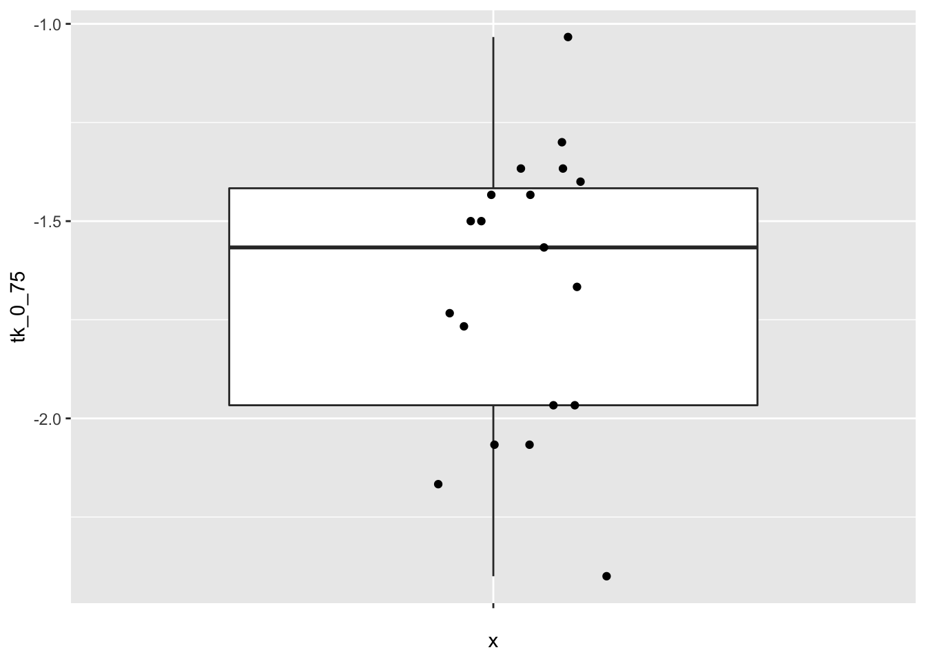

The data seems to plausibly come from a normal distribution, there don’t seem to be any outliers, and independence is not in question.

We will construct a 98% confidence interval for the change in temperature of the form $(-\infty, R)$. We will say that we are 98% confident that the treatment results in a temperature change of at most $R$ degrees Celsius. As before, this interval will be constructed so that 98% of the time that we perform the experiment, the true mean will fall in the interval (and 2% of the time, it will not). As before, we are assuming normality of and independent samples from the underlying population. We will also perform the following hypothesis test:

$H_0: \mu \ge 0$ vs.
$H_a: \mu < 0$

There is no difference in how we would run the test between $H_0: \mu \ge 0$ and $H_0: \mu = 0$ in this case, but knowing the alternative is $\mu < 0$ makes a difference. Now, the evidence that is least likely under $H_0$ (and most in favor of $H_a$) is all of the form $\overline{x} < R$. So, the percent of time we would make a reject $H_0$ when it is true is

\[ P(\frac{\overline{X} - \mu_0}{S/\sqrt{n}} < R) \]

where $\mu_0 = 0$ in this case. After collecting data, if we reject $H_0$, we would also have rejected $H_0$ if we got more compelling evidence against $H_0$, so we would compute

\[ P(t_{n-1} > \frac{\overline{x} - \mu_0}{S/\sqrt{n}}) \]

where $\frac{\overline{x} - \mu_0}{S/\sqrt{n}}$ is the value computed from the data. R does all of this for us:

t.test(cows_small$tk_0_75, mu = 0, alternative = "less", conf.level = .98)

## 
##  One Sample t-test
## 
## data:  cows_small$tk_0_75
## t = -20.509, df = 18, p-value = 3.119e-14
## alternative hypothesis: true mean is less than 0
## 98 percent confidence interval:
##       -Inf -1.488337
## sample estimates:
## mean of x 
## -1.668421

The confidence interval for the change in temperature associated with nozzle TK-0.75 is $(-\infty, -1.49)$ degrees Celsius. That is, we are 98 percent confident that the mean drop in temperature is at least 1.49 degrees Celsius. The $p$-value associated with the hypothesis test is $p = 3.1 \times 10^{-14}$, so we would reject $H_0$ that the mean temperature change is zero. We conclude that use of nozzle TK-0.75 is associated with a mean drop in temperature after three minutes as measured at the shoulder of the cows.

8.5 Assessing robustness via simulation

In the chapter up to this point, we have assumed that the underlying data is a random sample from a normal distribution. Let’s look at how various types of departures from those assumptions affect the validity of our statistical procedures. For the purposes of this discussion, we will restrict to hypothesis testing at a specified $\alpha$ level, but our results will hold for confidence intervals and reporting $p$-values just as well.

Our point of view is that if we design our hypothesis test at the $\alpha = .1$ level, say, then we want to incorrectly reject the null hypothesis 10% of the time. That is how our test is designed. In order to talk about this, we introduce some new terminology.

Definition 8.12

For a hypothesis test, a type I error is rejecting the null hypothesis when it is, in fact, true. The effective type I error rate of a hypothesis test is the probability that a type I error will occur.

When all of the assumptions of a hypothesis test at the $\alpha$ level are met, the effective type I error rate is exactly $\alpha$. If one or more of the assumptions are violated, then we want to estimate the
effective type I error rate and compare it to $\alpha$. If the new error rate is far from $\alpha$, then the test is not performing as designed. We will note whether the test makes too many type I errors or too few, but the main objective is to see whether the test is performing as designed.

Our first observation is that when the sample size is large, then the Central Limit Theorem tells us that $\overline{X}$ is approximately normal. Since $t_n$ is also approximately normal when $n$ is large, this gives us some measure of protection against departures from normality in the underlying population. It will be very useful to pull out the $p$-value of the t.test. Let’s see how we can do that. We begin by doing a t.test on “garbage data” just to see what t.test returns.

str(t.test(c(1, 2, 3)))

## List of 10
##  $ statistic  : Named num 3.46
##   ..- attr(*, "names")= chr "t"
##  $ parameter  : Named num 2
##   ..- attr(*, "names")= chr "df"
##  $ p.value    : num 0.0742
##  $ conf.int   : num [1:2] -0.484 4.484
##   ..- attr(*, "conf.level")= num 0.95
##  $ estimate   : Named num 2
##   ..- attr(*, "names")= chr "mean of x"
##  $ null.value : Named num 0
##   ..- attr(*, "names")= chr "mean"
##  $ stderr     : num 0.577
##  $ alternative: chr "two.sided"
##  $ method     : chr "One Sample t-test"
##  $ data.name  : chr "c(1, 2, 3)"
##  - attr(*, "class")= chr "htest"

It’s a list of 9 things, and we can pull out the $p$-value by using t.test(c(1,2,3))$p.value.

8.5.1 Symmetric, light tailed

Example Estimate the effective type I error rate in a t-test of $H_0: \mu = 0$ versus $H_a: \mu\not = 0$ at the $\alpha = 0.1$ level when the underlying population is uniform on the interval $(-1,1)$ when we take a sample size of $n = 10$.

Note that $H_0$ is definitely true in this case. So, we are going to estimate the probability of rejecting $H_0$ under the scenario above, and compare it to 10%, which is what the test is designed to give. Let’s build up our replicate function step by step.

set.seed(1)
runif(10, -1, 1) # Sample of size 10 from uniform rv

##  [1] -0.4689827 -0.2557522  0.1457067  0.8164156 -0.5966361  0.7967794
##  [7]  0.8893505  0.3215956  0.2582281 -0.8764275

t.test(runif(10, -1, 1))$p.value # p-value of test

## [1] 0.5089686

t.test(runif(10, -1, 1))$p.value < .1 # true if we reject

## [1] FALSE

mean(replicate(10000, t.test(runif(10, -1, 1))$p.value < .1))

## [1] 0.1007

Our result is 10.07%. That is really close to the designed value of 10%.

Tryit 8.3

Repeat the above example for various values of $\alpha$ and $n$. How big does $n$ need to be for the t.test to give results close to how it was designed? (Note: there is no one right answer to this ill-posed question! There are, however, wrong answers. The important part is the process you use to investigate.)

8.5.2 Skew

Example 8.13

Estimate the effective type I error rate in a t-test of $H_0: \mu = 1$ versus $H_a: \mu\not = 1$ at the $\alpha = 0.05$ level when the underlying population is exponential with rate 1 when we take a sample of size $n = 20$.

set.seed(2)
mean(replicate(20000, t.test(rexp(20, 1), mu = 1)$p.value < .05))

## [1] 0.08305

Note that we have to specify the null hypothesis mu = 1 in the t.test. Here we get an effective type I error rate (rejecting $H_0$ when $H_0$ is true) that is 3.035 percentage points higher than designed. This means our error rate will increase by 61%. Most people would argue that the test is not working as designed.

One issue is the following: how do we know we have run replicate enough times to get a reasonable estimate for the probability of a type I error? Well, we don’t. If we repeat our experiment a couple of times, though, we see that we get consistent results, which for now we will take as sufficient evidence that our estimate is closer to correct.

mean(replicate(20000, t.test(rexp(20, 1), mu = 1)$p.value < .05))

## [1] 0.08135

mean(replicate(20000, t.test(rexp(20, 1), mu = 1)$p.value < .05))

## [1] 0.0836

Pretty similar each time. That’s reason enough to believe the true type I error rate is relatively close to what we computed.

We summarize the simulated effective type I error rates for $H_0: \mu = 1$ versus $H_a: \mu \not= 1$ at $\alpha = .1, .05, .01$ and $.001$ levels for sample sizes $N = 10, 20, 50, 100$ and 200.

effectiveError <- sapply(c(.1, .05, .01, .001), function(y) {
  sapply(c(10, 20, 50, 100, 200), function(x) {
    mean(replicate(20000, t.test(rexp(x, 1), mu = 1)$p.value < y))
  })
})
colnames(effectiveError) <- c(".1", ".05", ".01", ".001")
rownames(effectiveError) <- c("10", "20", "50", "100", "200")
effectiveError

##          .1     .05     .01   .001
## 10  0.14845 0.10070 0.04455 0.0154
## 20  0.12640 0.07960 0.03360 0.0119
## 50  0.11300 0.06420 0.02275 0.0060
## 100 0.10735 0.05900 0.01610 0.0044
## 200 0.10400 0.05505 0.01325 0.0025

Tryit 8.4

Repeat the above example for exponential rv’s when you have a sample size of 150 for $\alpha = .1$, $\alpha = .01$ and $\alpha = .001$. We recommend increasing the number of times you are replicating as $\alpha$ gets smaller. Don’t go crazy though, because this can take a while to run.

From the previous exercise, you should be able to see that at $n = 50$, the effective type I error rate gets worse in relative terms as $\alpha$ gets smaller. (For example, my estimate at the $\alpha = .001$ level is an effective error rate more than 6 times what is designed! We would all agree that the test is not performing as designed.) That is unfortunate, because small $\alpha$ are exactly what we are interested in! That’s not to say that t-tests are useless in this context, but $p$-values should be interpreted with some level of caution when there is thought that the underlying population might be exponential. In particular, it would be misleading to report a $p$-value with 7 significant digits in this case, as R does by default, when in fact it is only the order of magnitude that is important. Of course, if you know your underlying population is exponential before you start, then there are techniques that you can use to get accurate results which are beyond the scope of this textbook.

8.5.3 Heavy tails and outliers

If the results of the preceding section didn’t convince you that you need to understand your underlying population before applying a t-test, then this section will. A typical “heavy tail” distribution is the $t$ random variable. Indeed, the $t$ rv with 1 or 2 degrees of freedom doesn’t even have a finite standard deviation!

Example 8.14

Estimate the effective type I error rate in a t-test of $H_0: \mu = 0$ versus $H_a: \mu\not = 0$ at the $\alpha = 0.1$ level when the underlying population is $t$ with 3 degrees of freedom when we take a sample of size $n = 30$.

mean(replicate(20000, t.test(rt(30, 3), mu = 0)$p.value < .1))

## [1] 0.0977

Not too bad. It seems that the t-test has an effective error rate less than how the test was designed.

Example 8.15

Estimate the effective type I error rate in a t-test of $H_0: \mu = 3$ versus $H_a: \mu\not = 3$ at the $\alpha = 0.1$ level when the underlying population is normal with mean 3 and standard deviation 1 with sample size $n = 100$. Assume, however, that there is an error in measurement, and one of the values is multiplied by 100 due to a missing decimal point.

mean(replicate(20000, {
  dat <- c(rnorm(99, 3, 1), 100 * rnorm(1, 3, 1))
  t.test(dat, mu = 3)$p.value < .1
}))

## [1] 3e-04

These numbers are so small, it makes more sense to sum them:

sum(replicate(20000, {
  dat <- c(rnorm(99, 3, 1), 100 * rnorm(1, 3, 1))
  t.test(dat, mu = 3)$p.value < .1
}))

## [1] 6

So, in this example, you see that we would reject $H_0$ 6 out of 20,000 times, when the test is designed to reject it 2,000 times out of 20,000! You might as well not even bother running this test, as you are rarely, if ever, going to reject $H_0$ even when it is false.

Example 8.16

Estimate the percentage of time you would correctly reject $H_0: \mu = 7$ versus $H_a: \mu\not = 7$ at the $\alpha = 0.1$ level when the underlying population is normal with mean 3 and standard deviation 1 with sample size $n = 100$. Assume, however, that there is an error in measurement, and one of the values is multiplied by 100 due to a missing decimal point.

Note that here, we have a null hypothesis that is 4 standard deviations away from the true null hypothesis. That should be easy to spot. Let’s see.

sum(replicate(20000, {
  dat <- c(rnorm(99, 3, 1), 100 * rnorm(1, 3, 1))
  t.test(dat, mu = 7)$p.value < .1
}))

## [1] 1457

There is no “right” value to compare this number to. We have estimated the probability of correctly rejecting a null hypothesis that is 4 standard deviations away from the true value (which is huge!!) as 0.0722. So, we would only detect a difference that large about 7% of the time that we run the test. That’s hardly worth doing.

8.5.4 Independence

There are two common types of dependence that we will investigate via simulations. One is when the sample consists of repeated measures on a common observational unit, and the other is when there is dependence between observations when ordered by another variable such as time. We only do simulations in the one-sample test of means.

Example 8.17

First, suppose that the experimental design consists of multiple measurements from a single unit. For example, we might measure the temperature of 20 people five times each in order to determine the mean temperature of healthy adults. In this case, it would be a mistake to assume that the observations are independent.

We suppose for the sake of argument that the true mean temperature of healthy adults is 98.6 with a standard deviation of 0.7. We model repeated samples as follows. First, choose a mean temperature for each of the 20 people, assume that healthy human temperatures follow a normal distribution with mean 98.6 and standard deviation 0.7. Then, assume that each person’s own temperatures are centered at their personal mean temperature with standard deviation 0.5.

# choose a mean temperature for each person
people_means <- rnorm(20, 98.6, .7)
# take five readings of each person
temps <- rnorm(100, mean = rep(people_means, 5), sd = 0.5)
glimpse(temps)

##  num [1:100] 97.9 99.3 99 99.2 98 ...

Now replicate this simulation to estimate the type I error rate:

sim_data <- replicate(1000, {
  people_means <- rnorm(20, 98.6, .7)
  temps <- rnorm(100, mean = rep(people_means, 5), sd = 0.5)
  t.test(temps, mu = 98.6)$p.value
})
mean(sim_data < .05)

## [1] 0.305

The effective type I error rate in this case is much larger than 5 percent! This is strong evidence that one should not ignore this type of dependence in ones data.

Tryit 8.5

Change the standard deviation from 0.7 to 2. Does the effective type I error rate to increase or decrease?
Now change the other standard deviation fro 0.5 to 2 (while returning the original standard deviation to 0.7). Does the effective type I error rate increase or decrease?
Return the standard deviations to 0.7 and 0.5, and now take 10 readings from 10 different people. What happens to the effective type I error rate?

Example 8.18

In the next example, we see what happens when there is a dependence between adjacent observations when ordered by a second variable. A common special case is when the observations are ordered via time. For example, if you wish to determine whether the high temperatures in a specific city in 2020 are higher than the were in 2000, you could subtract the high temperatures in 2000 from those in 2020. The resulting data would likely be dependent on time in the sense that if it was warmer on Feb 1 in 2020, then it will likely also be warmer on Feb 2 in 2020.

In order to simulate this, we will create 100 data points $x_1, \ldots, x_{100}$ such that $x_1$ is standard normal, and $x_n = 0.5 x_{n - 1} + z_n$, where $z_n$ is again standard normal. We see that the $n$th data point will depend on the previous data point relatively strongly, and on ones before that to a smaller extent.

We show two ways to simulate data of this type. The first uses a while loop, which we only covered briefly in the “Loops in R” Vignette at the end of Chapter 5. Readers who do not wish to see this can safely bypass to the built in R function which samples from this distribution.

x <- rep(NA, 100) # create a vector of length 100 that we will fill in below
x[1] <- rnorm(1)
i <- 2
while (i < 101) {
  x[i] <- .5 * x[i - 1] + rnorm(1)
  i <- i + 1
}
plot(x, type = "l")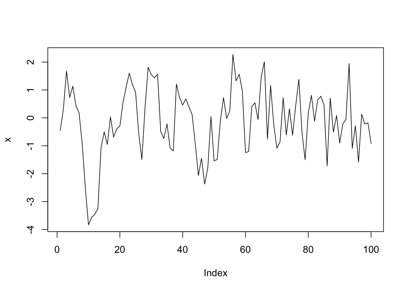

This is a common enough process that there is a built in R function arima.sim which does essentially this and much, much more. For our purposes, we only care about the ar parameter in the model list. That is the value $c$ such that $x_n = c x_{n - 1} + z_n$.

x <- arima.sim(model = list(ar = .5), n = 100)

Now we suppose that we have data of this type, and we estimate the effective type I error rate when testing $H_0: \mu = 0$ versus $H_a: \mu \not= 0$.

sim_data <- replicate(10000, {
  x <- arima.sim(model = list(ar = .5), n = 100)
  t.test(x, mu = 0)$p.value
})
mean(sim_data < .05)

## [1] 0.2565

Again, we see that we have an effective type I error rate much higher than the desired rate of $\alpha = .05$. It would be inappropriate to use t.test in this way on data of this type.

Tryit 8.6

Change the ar parameter to .1 and to .9 and estimate the effective type I error rate. Which one is performing closest to the desired rate of $\alpha = .05$?

8.5.5 Summary

When doing t-tests on populations that are not normal, the following types of departures from design were noted.

When the underlying distribution is skew, the exact $p$-values should not be reported to many significant digits (especially the smaller they get). If a $p$-value close to the $\alpha$ level of a test is obtained, then we would want to note the fact that we are unsure of our $p$-values due to skewness, and fail to reject.
When the underlying distribution has outliers, the power of the test is severely compromised. A single outlier of sufficient magnitude will force a t-test to never reject the null hypothesis. If your population has outliers, you do not want to use a t-test.
When the sample is not independent, then the source and type of dependence will need to be understood and adjusted for. It is not typically appropriate to use t.test without making these adjustments.

8.6 Two sample hypothesis tests

This section presents hypothesis tests for comparing the means of two populations. In this situation, we have two populations that we are sampling from, and we ask whether the mean of population one differs from the mean of population two.

For tests of the mean, we must assume the underlying populations are normal, or that we have enough samples so that the Central Limit Theorem takes hold. We are also as always assuming that there are no outliers. Remember: outliers can kill $t$ tests. Both the one-sample and the two-sample variety.

For two sample tests, the (unknown) means of the two populations are $\mu_1$ and $\mu_2$. Our hypotheses are:

$H_0: \, \mu_1 = \mu_2$ versus

$H_a: \, \mu_1 \not= \mu_2$.

As with one sample tests, the alternate hypothesis may be one sided if justified by the experiment. One sided tests have $H_a: \mu_1 \leq \mu_2$ or $H_a: \mu_1 \geq \mu_2$. To use one sided tests, the experimenter should have a compelling and pre-existing reason to be sure $H_a$ is true whenever $H_0$ is false.

The most straightfoward experiment that results in two independent samples is a study comparing the same measurement on two different populations. In this case, a sample is chosen from population one, a second sample is chosen independently from population two, and both samples are measured. Another common setting is a controlled experiment. In a controlled experiment, the two populations are a group that receives some treatment and a control group that does not⁵⁴. Subjects are randomly assigned to either the control or treatment group. In both of these designs, the two independent samples $t$-test is appropriate.

The two sample paired $t$-test is used when data comes in pairs. Pairs may be two different subjects matched for some common traits, or they may come from two measurements on a single subject.

For example, suppose you wish to determine whether a new fertilizer increases the mean number of apples that apple trees produce. Here are three reasonable experimental designs:

Design 1. Randomly select two samples of trees. Apply fertilizer to one sample and leave the other sample alone as a control group. At the end of the growing season, count the apples on each tree in each group.
Design 2. Choose one sample of trees for the experiment. Count the number of apples on each tree after one growing season. The next season apply the fertilizer and count the number of apples again.
Design 3. Carefully choose trees in pairs, so that each pair of trees is of similar maturity and will grow under similar conditions (soil quality, water, sunlight). Randomly assign one tree of each pair to receive fertilizer and the other to act as control. Count the number of apples on the fertilized trees and the unfertilized trees.

Photo credit: George Chernilevsky

In design 1, the two independent samples $t$-test is appropriate. Data from this experiment will likely be in long form, with a two-valued grouping variable in one column and a measurement variable giving apple counts in a second column, as in the first table in Table 8.2.

Designs 2 and 3 result in paired data. The measures in the two populations are dependent. You expect there to be some relationship between the number of apples you count on each pair. For example, big trees would have more apples each season than small trees. In general, it is a hard problem to deal with dependent data, but paired data is a dependency we can handle with the two sample paired $t$-test.

In designs 2 and 3, the data will likely be in wide form for analysis: each row representing a pair, and two columns with apple counts. In design 2, the rows are individual trees and the columns are the two measurements, before and after. In design 3, the rows are pairs of trees and the columns are measurements for the fertilized and unfertilized member of each pair. See Table 8.2.

Table 8.2: Data from three expermental designs: independent samples, before/after, and matched pairs.

group	apples
fertilized	660
control	533
fertilized	418
fertilized	549
control	574
fertilized	558

before	after
469	496
651	498
539	594
438	582
279	559
612	592

fertilized	control
578	353
507	452
301	542
562	636
494	490
484	539

8.6.1 Two independent samples $t$-test

For the two independent samples $t$-test, we require data $x_{1,1},\dotsc,x_{1,n_1}$ drawn from one population and $x_{2,1},\dotsc,x_{2,n_2}$ drawn independently from a second population.

Assumptions 8.2

The samples are independent
The underlying populations are normal or the sample sizes are large.
There are no outliers.

We calculuate the means of the two samples $\overline{x}_1$ and $\overline{x}_2$ and their variances $s_1^2$ and $s_2^2$. The test statistic is given by

\[ t = \frac{\overline{x}_1 - \overline{x}_2}{\sqrt{s_1^2/n_1 + s_2^2/n_2}}. \]

If the assumptions are met, then the test statistic has a $t$ distribution with a complicated (and non-integer) df. In the past, when computations like this were made by hand, it was common to add an additional assumption of “equal variances” so that $s_1^2 = s_2^2$ and the expression for $t$ simplifies somewhat. In general, it is a more conservative approach not to assume the variances of the two populations are equal, and we generally recommend not to assume equal variance unless you have a good reason for doing so.

In R, the two independent samples $t$-test is performed with the syntax t.test(value ~ group, data=dataset). Here value is the name of the measurement variable, group should be a variable that takes on exactly two values, and dataset is the name of the dataset. The value ~ group expression is known as a formula, and should be read as “value which depends on group”. We will see this syntax used frequently in Chapter 11 when performing regression analysis.

Example 8.19

We return to the brake data in the fosdata package. Recall that we were interested in whether there is a difference in the mean time for an older person and the mean time for a younger person to release the brake pedal after it unexpectedly causes the car to speed up.

Let $\mu_1$ be the mean time to release the pedal for the older group, and let $\mu_2$ denote the mean time of the younger group in ms.

\[ H_0: \mu_1 = \mu_2 \] versus \[ H_a: \mu_1\not= \mu_2 \]

It might be reasonable to do a one-sided test here if you have data or other evidence suggesting that older drivers are going to have slower reaction times, but we will stick with the two-sided tests.

Let’s think about the data that we have for a minute. Do we expect the reaction times to be approximately normal? How many samples do we have? We compute the mean, sd, skewness and number of observations in each group and also plot the data.

brake <- fosdata::brake
brake %>%
  group_by(age_group) %>%
  summarize(
    mean = mean(latency_p2),
    sd = sd(latency_p2),
    skew = e1071::skewness(latency_p2),
    N = n()
  )

## # A tibble: 2 x 5
##   age_group  mean    sd  skew     N
##   <chr>     <dbl> <dbl> <dbl> <int>
## 1 Old        956. 242.  1.89     40
## 2 Young      664.  95.9 0.780    40

ggplot(brake, aes(x = age_group, y = latency_p2)) +
  geom_boxplot(outlier.size = -1) +
  geom_jitter(height = 0, width = .2)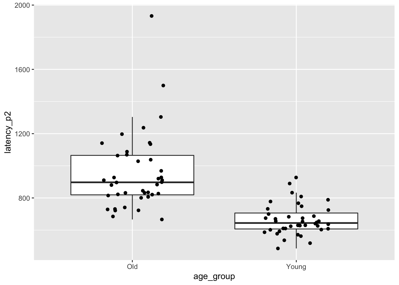

The older group in particular is right skew, and there is one extreme outlier among the older drivers. These are concerns, but with 80 observations our assumptions are met well enough. We tell t.test to break up latency_p2 by age_group and perform a two-sample t-test.

t.test(latency_p2 ~ age_group, data = brake)

## 
##  Welch Two Sample t-test
## 
## data:  latency_p2 by age_group
## t = 7.0845, df = 50.97, p-value = 4.014e-09
## alternative hypothesis: true difference in means is not equal to 0
## 95 percent confidence interval:
##  208.7430 373.8345
## sample estimates:
##   mean in group Old mean in group Young 
##            955.7747            664.4859

We reject the null hypothesis that the two means are the same ($p = 4.0 \times 10^{-9}$). A 95 percent confidence interval for the difference in mean times is $[209, 374]$ ms. That is, we are 95 percent confident that the mean time for older drivers is between 209 and 374 ms slower than the mean time for younger drivers.

In Exercise 8.35, you are asked to redo this analysis after removing the largest older driver outlier. When doing so, you will see that the skewness is improved, the $p$-value gets smaller, and the confidence interval gets more narrow. Therefore, we have no reason to doubt the validity of the work we did with the outlier included.

Tryit 8.7

Is there a significant difference between young and old drivers in the mean time to press the brake after seeing the red light (latency_p1)?

8.6.2 Paired two sample $t$-test

For the paired two-sample $t$-test, we require data $x_{1,1},\dotsc,x_{1,n}$ drawn from one population and $x_{2,1},\dotsc,x_{2,n}$ drawn from a second population. The data come in pairs, so that $x_{1,i}$ and $x_{2,i}$ are not independent.

Assumptions 8.3

The samples are paired
The underlying populations are normal or the sample size is large.
There are no outliers.

It makes sense to compute the difference $d_i = x_{1,i} - x_{2,i}$ for each pair. Then we simply perform a one-sample $t$ test to test the differences against zero. The mean and variance of $d$ are $\overline{d} = \overline{x}_1 + \overline{x}_2$ and $s_d^2$. So the test statistic is

\[ t = \frac{\overline{x}_1 - \overline{x}_2}{s_d/\sqrt{n}}. \]

When the test assumptions are met, this will have the $t$ distribution with $n-1$ df.

In R, the syntax for a paired $t$-test is t.test(dataset$var1, dataset$var2, paired=TRUE).

Alert 8.4

It is possible to perform a paired $t$-test on long format data with formula notation value ~ group. This requires you to be sure that the data pairs are in order. More often than not, long format data is unpaired and using formula notation to perform a paired test is a mistake.

Example 8.20

Return to the cows_small data set in the fosdata package. We wish to determine whether there is a difference between nozzle TK-0.75 and nozzle TK-12 in terms of the mean amount that they cool down cows in a three minute period.

Let $\mu_1$ denote the mean change in temperature of cows sprayed with TK-0.75 and let $\mu_2$ denote the mean change in temperature of cows sprayed with TK-12. Our null hypothesis is $H_0: \mu_1 = \mu_2$ and our alternative is $H_a: \mu_1\not= \mu_2$. According to the manufacturer of the TK-0.75, it sprays 0.4 liters per minute at 40 PSI, while the TK-12 sprays 4.5 liters per minute. Since the TK-12 sprays considerably more water, it would be worth considering a one-sided test in this case. However, we don’t know any other characteristics of the nozzles which might mitigate the flow advantage of the TK-12, so we stick with a two-sided test.

The data is in wide format, with one column for each nozzle type. To check assumptions, we compute and plot the difference variable. Here we chose to use a qq plot but a histogram or boxplot would have also been appropriate.

cows_small <- fosdata::cows_small
ggplot(cows_small, aes(sample = tk_0_75 - tk_12)) +
  geom_qq() +
  geom_qq_line()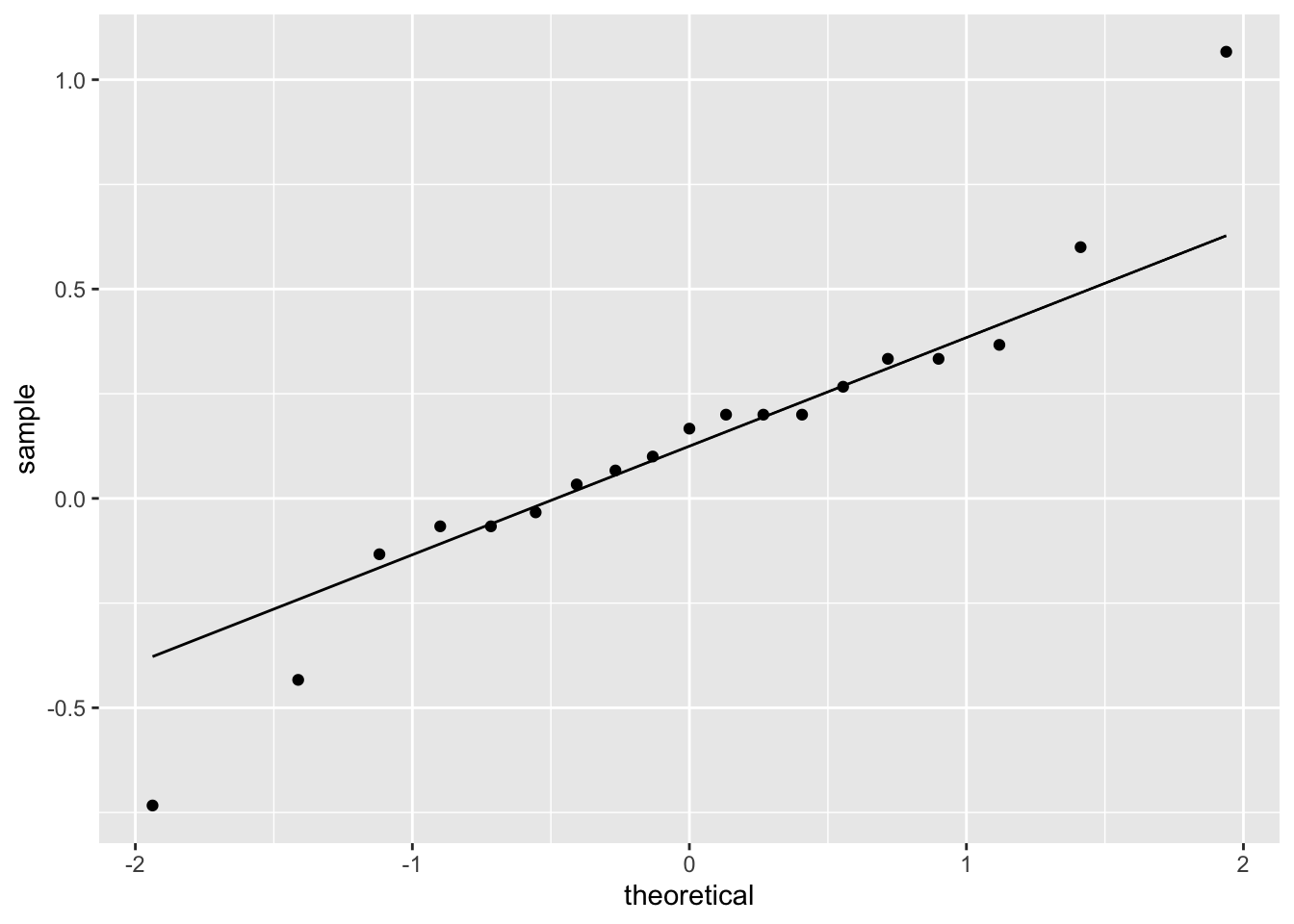

The distribution is somewhat heavy-tailed but good enough to proceed. We perform the paired two sample $t$-test.

t.test(cows_small$tk_12, cows_small$tk_0_75, paired = TRUE)

## 
##  Paired t-test
## 
## data:  cows_small$tk_12 and cows_small$tk_0_75
## t = -1.5118, df = 18, p-value = 0.1479
## alternative hypothesis: true difference in means is not equal to 0
## 95 percent confidence interval:
##  -0.31023781  0.05058868
## sample estimates:
## mean of the differences 
##              -0.1298246

We find a 95 percent confidence interval for the difference in the means to be $[-0.31, 0.05]$, and we do not reject $H_0$ at the $\alpha = .05$ level ($p$ = .1479). We cannot conclude that there is a difference in the mean temperature change associated with the two nozzles.

Tryit 8.8

Is there a significant difference in the mean teperature change between the TK-0.75 nozzle and the control?

8.7 Type II errors and power

Up to this point, we have been concerned about the probability of rejecting the null hypothesis when the null hypothesis is true. There is another type of error that can occur, however, and that is failing to reject the null hypothesis when the null hypothesis is false.

Definition 8.21

A type I error is rejecting the null when it is true.
A type II error is failing to reject the null when it is false.

Definition 8.22

The power of a test is defined to be one minus the probability of a type II error, which is the probability of correctly rejecting the null hypothesis.

One issue that arises is that the null hypothesis is (usually) a simple hypothesis; that is, it consists of a complete specification of parameters, while the alternative hypothesis is often a composite hypothesis; that is, it consists of parameters in a range of values. Therefore, when we say the null hypothesis is false, we are not completely specifying the distribution of the population. For this reason, the type II error is a function that depends on the value of the parameter(s) in the alternative hypothesis.

Let’s look at the heart rate example using normtemp. Suppose that our null hypothesis is that the mean heart rate of healthy adults is 80 beats per minute. (The American Heart Association says normal is from 60-100.) Our alternative hypothesis is that the mean heart rate of healthy adults is not 80 beats per minute. We take a sample of size 130. What is the probability of a type II error? Well, we can’t do that yet, because we don’t know the standard deviation of the underlying population or the $\alpha$ level of the test. Since the range of values according to AHA is between 60 and 100, which we interpret to mean that about 99% of healthy adults will fall in this range, we will estimate the standard deviation to be (100 - 60)/6 = 6.67. Next, we will fix a value for the alternative hypothesis. Let’s compute the probability of a type II error when the true mean is 78 beats per minute.

It is possible to do this by hand using the non-central parameter ncp argument of pt, but let’s do it using simulation. We start by taking a sample of size 130 from a normal distribution with mean 78 and standard deviation 6.67. We compute the t statistic and determine whether we would reject $H_0$. We assume $\alpha = .01$.

dat <- rnorm(130, 78, 6.67)
t_stat <- (mean(dat) - 80) / (sd(dat) / sqrt(130))
t_stat

## [1] -3.843193

qt(.005, 129) # critical value

## [1] -2.614479

Since t_stat is less than qt(.005, 129) we would (correctly) reject the null hypothesis. Easier would be to use the built in R function t.test to perform the test.

dat <- rnorm(130, 78, 6.67)
t.test(dat, mu = 80)$p.value > .01

## [1] FALSE

Next, we compute the percentage of times that the $p$-value of the test is greater than .01. That is the percentage of times that we have made a type II error, and will be our estimate for the probability of a type II error.

simdata <- replicate(10000, {
  dat <- rnorm(130, 78, 6.67)
  t.test(dat, mu = 80)$p.value > .01
})
mean(simdata)

## [1] 0.2115

We get about a 0.2115 chance for a type II error in this case.

There is a built-in R function which will make this computation for you, called power.t.test. It has the following arguments:

n the number of samples
delta the difference between the null and alternative mean
sd the standard deviation of the population
sig.level the $\alpha$ significance level of the test
power this is one minus the probability of a type II error
type either one.sample, two.sample or paired, default is two
alternative two.sided or one.sided, default is two

The function works by specifying four of the first five parameters, and the function then solves for the unspecified parameter. For example, if we wish to re-do the above simulation using power.t.test, we would use the following.

power.t.test(
  n = 130, delta = 2, sd = 6.67,
  sig.level = .01, type = "one"
)

## 
##      One-sample t test power calculation 
## 
##               n = 130
##           delta = 2
##              sd = 6.67
##       sig.level = 0.01
##           power = 0.7878322
##     alternative = two.sided

The power is 0.7878322, so the probability of a type II error is one minus that, or

1 - .7878322

## [1] 0.2121678

which is close to what we computed in the simulation.

A traditional approach in designing experiments is to specify the significance level and power, and use a simulation or power.t.test to determine what sample size is necessary to achieve that power. In order to do so, we must estimate the standard deviation of the underlying population and we must specify the effect size that we are interested in. Sometimes there is an effect size in the literature that can be used. Other times, we can pick a size that would be clinically significant (as opposed to statistically significant). Think about it like this: if the true mean body temperature of healthy adults is 98.59, would that make a difference in treatment or diagnosis? No. What about if it were 100? Then yes, that would make a difference in diagnoses! It is subjective and can be challenging to specify what delta to provide, but we should provide one that would make an important difference in some context.

Let’s look at the body temperature study. We have as our null hypothesis that the mean temperature of healthy adults is 98.6 degrees. We estimate the standard deviation of the underlying population to be 0.3 degrees. After consulting with our subject area expert, we decide that a clinically significant difference from 98.6 degrees would be 0.2 degrees. That is, if the true mean is 98.4 or 98.8 then we want to detect it with power 0.8. The sample size needed is

power.t.test(
  delta = 0.2, sd = .3,
  sig.level = .01, power = 0.8, type = "one"
)

## 
##      One-sample t test power calculation 
## 
##               n = 29.64538
##           delta = 0.2
##              sd = 0.3
##       sig.level = 0.01
##           power = 0.8
##     alternative = two.sided

We would need to collect 30 samples in order to have an appropriately powered test.

8.7.1 Effect size

We used the word “effect size” above, without really saying what we mean. A common measure of the effect size is given by Cohen’s $d$
\[ d = \frac{\overline{x} - \mu_0}{S}, \] the difference between the sample mean and the mean from the null hypothesis, divided by the sample standard deviation. The parametrization of power.t.test is redundant in the sense that the power of a test only relies delta and sd through the effect size $d$. As an example, we note that when delta = .1 and sd = .5 the effect size is 0.2, as it also is when delta = .3 and sd = 1.5. Both of these give the same power:

power.t.test(n = 30, delta = .3, sd = 1.5, sig.level = .05, type = "one")

## 
##      One-sample t test power calculation 
## 
##               n = 30
##           delta = 0.3
##              sd = 1.5
##       sig.level = 0.05
##           power = 0.1839206
##     alternative = two.sided

power.t.test(n = 30, delta = .1, sd = .5, sig.level = .05, type = "one")

## 
##      One-sample t test power calculation 
## 
##               n = 30
##           delta = 0.1
##              sd = 0.5
##       sig.level = 0.05
##           power = 0.1839206
##     alternative = two.sided

It is common to report the effect size, especially when there is statistical significance. The following chart gives easily interpretable values for $d$. The adjectives associated with effect size should be taken with a grain of salt, though, and they do not replace having a domain area understanding of effect.

Table 8.3: Descriptors of Effect Sizes
Effect Size	d
Very Small	0.01
Small	0.20
Medium	0.50
Large	0.80
Very Large	1.20

If you are designing an experiment and you aren’t sure what effect size to choose for power computation, you can use the descriptors to give yourself an idea of what size you want to detect, with the understanding that this varies widely between disciplines.

You do not want your test to be underpowered for two reasons. First, you likely will not reject the null hypothesis in instances where you would like to be able to do so. Second, when effect sizes are estimated using underpowered tests, they tend to be overestimated. This leads to a reproducibility problem, because when people design further studies to corroborate your study, they are using an effect size that is too high. Let’s run some simulations to verify. We assume that we have an experiment with power 0.2.

power.t.test(
  delta = 0.2, sd = 1, sig.level = .05,
  power = 0.25, type = "one"
)

## 
##      One-sample t test power calculation 
## 
##               n = 43.24862
##           delta = 0.2
##              sd = 1
##       sig.level = 0.05
##           power = 0.25
##     alternative = two.sided

This says when $d = 0.2$, we need 43 samples for the power to be 0.25. Remember, this is not recommended! We use simulation to estimate the percentage of times that the null hypothesis is rejected. We assume we are testing $H_0: \mu = 0$ versus $H_a: \mu \not=0$.

simdata <- replicate(10000, {
  dat <- rnorm(43, 0.2, 1)
  t.test(dat, mu = 0)$p.value
})
mean(simdata < .05)

## [1] 0.2438

And we see that indeed, we get about 25%, which is what power.t.test predicted. Note that the true effect size is 0.2. The estimated effect size from tests which are significant is given by:

simdata <- replicate(10000, {
  dat <- rnorm(43, 0.2, 1)
  ifelse(t.test(dat, mu = 0)$p.value < .05,
    abs(mean(dat)) / sd(dat),
    NA
  )
})
mean(simdata, na.rm = TRUE)

## [1] 0.408912

We see that the mean estimated effect size is double the actual effect size, so we have a biased estimate for effect size. If we have an appropriately powered test, then this bias is much less.

power.t.test(
  delta = 0.2, sd = 1, sig.level = .05,
  power = 0.8, type = "one"
)

## 
##      One-sample t test power calculation 
## 
##               n = 198.1513
##           delta = 0.2
##              sd = 1
##       sig.level = 0.05
##           power = 0.8
##     alternative = two.sided

simdata <- replicate(10000, {
  dat <- rnorm(199, 0.2, 1)
  ifelse(t.test(dat, mu = 0)$p.value < .05,
    abs(mean(dat)) / sd(dat),
    NA
  )
})
mean(simdata, na.rm = TRUE)

## [1] 0.2239006

Vignette: A permutation test

What do you do when you aren’t sure whether your data comes from a population that satisfies the assumptions of a $t$-test? One popular alternative is the permutation test . If we imagine that there was no difference between the two populations, then the assignments of the grouping variables can be considered random. A permutation test takes random permutations of the grouping variables, and re-computes the test statistic. Under $H_0$: the response is independent of the grouping, we should often get values as extreme as the value obtained in the sample. We reject $H_0$ if the proportion of times we get something as unusual as in the sample is less than $\alpha$/

Let’s consider the brake data that we studied in this chapter, except this time we consider latency_p1, the time for the subject to hit the brake after seeing a red light. Load the data with:

brake <- fosdata::brake

Next, we compute the mean latency for releasing the brake of the older group minus the mean of the younger group.

mean_Old <- mean(brake$latency_p1[brake$age_group == "Old"])
mean_Young <- mean(brake$latency_p1[brake$age_group == "Young"])
mean_brake <- mean_Old - mean_Young
mean_brake

## [1] -10.94183

The older group was on average a bit faster than the younger group. Let’s also look at a boxplot.

ggplot(brake, aes(x = age_group, y = latency_p1)) +
  geom_boxplot(outlier.size = -1) +
  geom_jitter(height = 0, width = 0.2)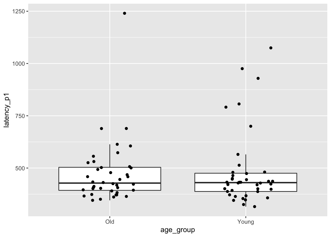

The data is visibly skew, so there should be at least some hesitation to use a $t$-test. Instead, we permute the age groups many times and recompute the test statistic.

perm_test <- replicate(10000, {
  # generate new randomly permuted age groups
  new_age_groups <- sample(brake$age_group)
  mean_Old <- mean(brake$latency_p1[new_age_groups == "Old"])
  mean_Young <- mean(brake$latency_p1[new_age_groups == "Young"])
  mean_Old - mean_Young
})
hist(perm_test)
abline(v = mean_brake, lty = 2)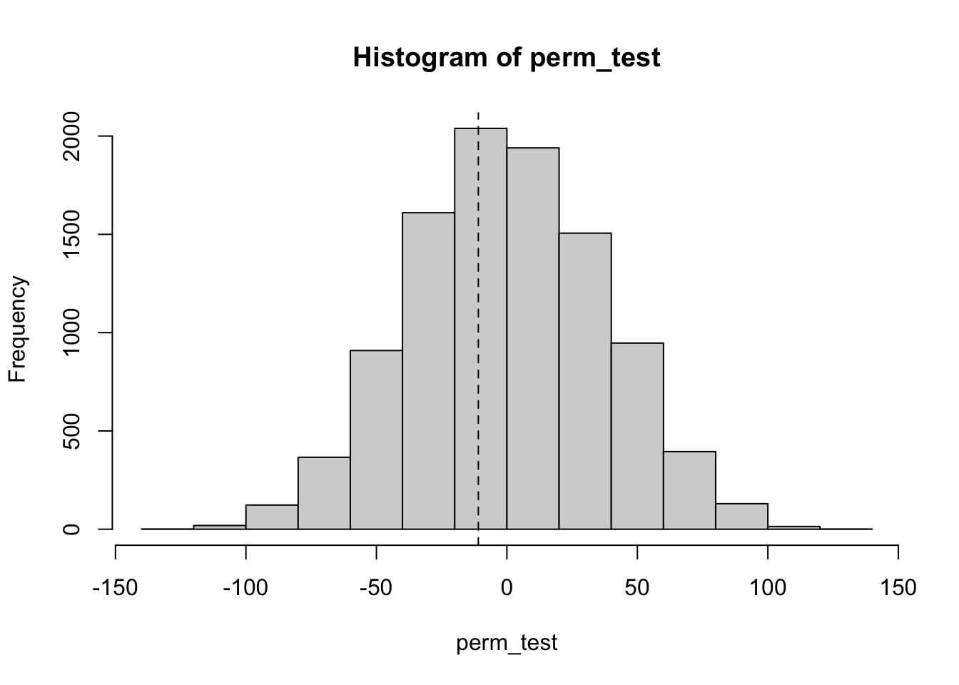

We see from the histogram that it is not at all unusual to get a value of $-10.9$. To get a $p$-value, we compute

2 * mean(perm_test < mean_brake)

## [1] 0.7914

We have a $p$-value of .8456, and we would not reject the null hypothesis. In the $p$-value computation, we only test for perm_test < mean_brake because mean_brake is negative. For a positive observation, the inequality would reverse.

Exercises

Exercises 8.1 - 8.5 require material through Section 8.1.

8.1

Let $X_1, \ldots, X_{12}$ be independent normal random variables with mean 1 and standard deviation 3. Confirm via simulation that \[ \frac{\overline{X} - 1}{3/\sqrt{12}} \] is $t$ with 11 degrees of freedom.

8.2

Let $a = 0$ and $b = 1$. Find a value of $n$ such that $\left|P(a < X_n < b) - P(a < Z < b)\right| < .01$, where $X_n$ is a $t$ random variable with $n$ degrees of freedom and $Z$ is a standard normal random variable.

8.3

Let $X$ be a $t$ random variable with 6 degrees of freedom. Find a constant $C > 0$ such that \[ P(-C < X < C) = .8 \]

8.4

Compute $P(z > 2)$, where z is the standard normal variable. Compute $P(t > 2)$ for $t$ having Student’s $t$ distribution with each of 40, 20, 10, and 5 degrees of freedom. How does the DF affect the area in the tail of the $t$ distribution?

8.5

Let $X_1, \ldots, X_{20}$ be independent normal random variables with mean 7 and unknown standard deviation. Find the value of $C$ such that \[ P(\overline{X} - C (S/ \sqrt{n}) < \mu < \overline{X} + C (S/ \sqrt{n})) = 0.99, \] where $S$ as usual is the sample standard deviation.

Exercises 8.6 - 8.13 require material through Section 8.2.

8.6

The data set fosdata::plastics gives measurements of plastic microfibers found in snow. Give the 99% confidence interval for the mean diameter of plastic microfibers.

8.7

The data set morley is built in to R. The Speed variable contains 100 measurements of the speed of light, conducted by A. A. Michelson in 1879. Measurements have 299000m/s subtracted from them.

Compute the 95% confidence interval for the speed of light. Does your confidence interval contain the modern accepted speed of light of 299729 m/s?

8.8

Consider the fosdata::brake data set discussed in the chapter. Recall that latency_p2 is the time it takes subjects to release the pedal once they have pressed it and the car has started to accelerate rather than decelerate. Find a 95% confidence interval for the P2 latency for young drivers based on the data.

8.9

The dataset fosdata::cows_small gives the change in shoulder temperature of cows standing in the heat.

Give the 95% confidence interval for the shoulder temperature change after spraying with the tk_12 nozzle.
Give the 95% confidence interval for the shoulder temperature change after no spraying (control).
Which of the two intervals is wider?
What is the standard deviation of temperature change for the tk_12 condition? For the control condition?
How are your answers to parts (c) and (d) related?

8.10

Suppose that $X_1, \ldots, X_5$ is a random sample from a normal distribution with unkown mean and known standard deviation 2. If $\overline{X} = 3$, then find a 95 percent confidence interval for the mean using the fact that $\frac{\overline{X} - \mu}{\sigma/\sqrt{n}}$ is a standard normal random variable.

8.11

Some data randomly sampled from a normal population has a sample mean of 30. Match each interval on the left with one of the descriptions on the right:

Interval	Description
a. [28.5, 31.5]	I. A 90% confidence interval.
b. [28.0, 32.0]	II. A 95% confidence interval.
c. [28.7, 31.3]	III. A 99% confidence interval.

8.12

Suppose you collect a random sample of size 20 from a normal population with unknown mean and standard deviation. Suppose $\overline{X} = 2.3$ and $S = 1.2$.

The interval $[2.0, 2.6]$ is a confidence interval for the mean. What percent confidence interval is it?
Find a 98 percent confidence interval for the mean.

8.13

Suppose a population has an exponential distribution with $\lambda = 0.5$. We can simulate drawing a sample of size 10 from this population with rexp(10,5) and compute a 95% confidence interval with t.test(rexp(10,.5),mu=2)$conf.int.

What is the population mean $\mu$?
Write code to simulate 10000 confidence intervals and determine what percent of the time $\mu$ is in the 95% confidence interval.
Why is your answer different from 95%?

Exercises 8.14 - 8.19 require material through Section 8.3.

8.14

Consider the react data set from ISwR. Find a 98% confidence interval for the mean difference in measurements of the tuberculin reaction. Does the mean differ significantly from zero according to a t-test? Interpret.

8.15

Suppose you collect a random sample of size 20 from a normal population with unknown mean and standard deviation. You wish to test $H_0: \mu = 2$ versus $H_a: \mu \not= 2$.

The region $|T| > 1.6$ is a rejection region for this hypothesis test. What is the $\alpha$ level of the rejection region?
Find a rejection region that corresponds to $\alpha = .005$.

Figure 8.2

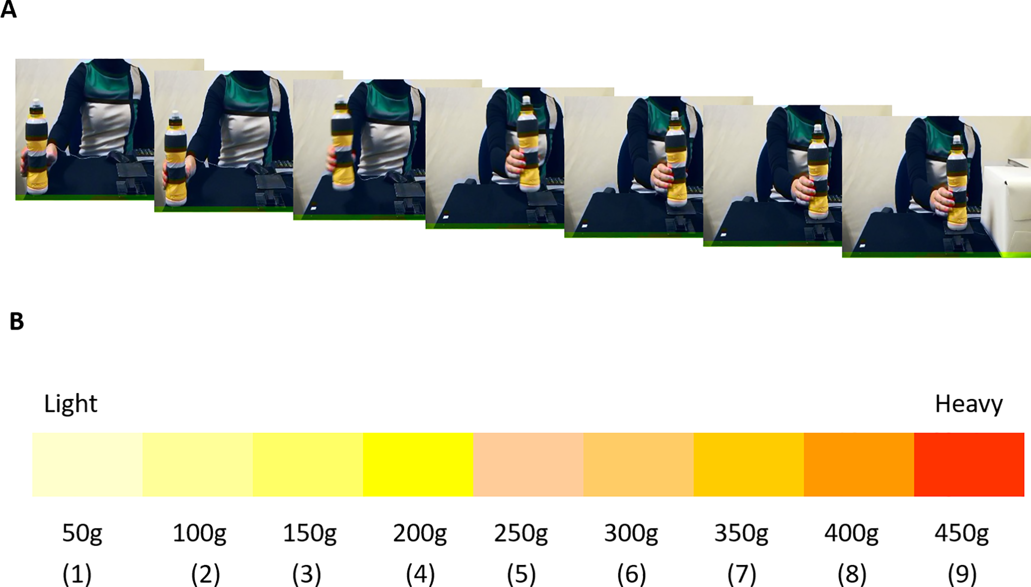
Figure 8.2: Figure from Alessandra, et al

8.16

The data fosdata::weight_estimate gives children’s estimates of weights lifted by actors.
State and carry out a hypothesis test that the mean of the children’s estimates of the 100g object differ from the actual weight, 100g. Repeat this test for the 200g, 300g, and 400g objects. Which of the estimates were significantly different from the correct weights?

8.17

Consider the bp.obese data set from ISwR. It contains data from a random sample of Mexican-American adults in a small California town. Consider only the blood pressure data for this problem. Normal diastolic blood pressure is 120. Is there evidence to suggest that the mean blood pressure of the population differs from 120? What is the population in this example?

8.18

Suppose we wish to test $H_0: \mu = 1$ versus $H_a: \mu\not= 1$. Let $X_1, \ldots, X_5$ be a random sample from a normal population with known standard deviation $\sigma = 2$. We construct the test statistic $Z = \frac{\overline{X} - 1}{\sigma/\sqrt{n}}$.

If the rejection region is $|Z| > 2.2$, then what is the significance level of the test?
What would a rejection region be that corresponds to a significance level of $\alpha = .01$?

8.19

For the ISwR::bp.obese data set, consider the obese variable. What is the natural null hypothesis? Is there evidence to suggest that the obesity level of the population differs from the null hypothesis?

Exercise 8.20 requires material through Section 8.4.

8.20

Suppose that a dishonest statistician is doing a $t$-test of $H_0: \mu = 0$ at the $\alpha = .05$ level. The statistician waits until he gets the data to specify the alternative hypothesis. If $\overline{X} > 0$, then they choose $H_a: \mu > 0$ and if $\overline{X} < 0$, they choose $H_a: \mu < 0$. Suppose the statistician collects 20 independent samples and the underlying population is standard normal. Use simulation to confirm that the null hypothesis is rejected 10 percent of the time.

Exercises 8.21 - 8.24 require material through Section 8.5.

8.21

This problem illustrates that t.test performs as expected when the underlying population is normal. a. Choose 10 random values of $X$ having the Normal(4, 1) distribution. Use t.test to compute the 95% confidence interval for the mean. Is 4 in your confidence interval? b. Replicate the experiment in part a 10,000 times and compute the percentage of times the population mean 4 was included in the confidence interval.

8.22

Mackowiak et al⁵⁵ studied the mean normal body temperature of healthy adults. One hundred forty-eight subjects’ body temperatures were measured one to four times daily for 3 consecutive days for a total of 700 temperature readings. Let $\mu$ denote the true mean normal body temperature of healthy adults and $X_1, \ldots, X_{700}$ the temperature readings from the study. Is it correct that \[ \frac{\overline{X} - \mu}{S/\sqrt{n}} \] is a $t$ random variable with 699 degrees of freedom?

8.23

This problem explores the accuracy of t.test when the underlying population is skew. a. Choose 10 random values of $X$ having an exponential distribution with rate 1/4. Use t.test to compute the 95% confidence interval for the mean. Is the true mean, 4, in your confidence interval? b. Replicate the experiment in part a 10,000 times and compute the percentage of times that the population mean 4 was included in the confidence interval. Explain why this number is not 95 percent. c. Repeat part b using 100 values of $X$ to make each confidence interval. What percentage of times did the confidence interval contain the population mean? Why is it closer to 95 percent?

8.24

This problem explores the accuracy of t.test when the data is not independent. Suppose $X_1, \ldots, X_{20}$ is a random sample from normal population with mean 0 and standard deviation 1. Let $Y_1 = X_1 + X_2$, $Y_2 = X_2 + X_3, \ldots,$ and $Y_{19} = X_{19} + X_{20}$. Note that $Y_1, \ldots, Y_{19}$ are not independent, but they do have mean 0. Estimate the effective type I error rate when testing $H_0: \mu = 0$ versus $H_a: \mu \not= 0$ at the $\alpha = .05$ level using $Y_1, \ldots, Y_{19}$. (Hint: convolve(X, c(1, 1), type = "filter") computes the sums of pairs of values of $X$ as described in this problem.)

Exercises 8.25 - 8.35 require material through Section 8.6.

8.25

Each of these studies has won the prestigious Ig Nobel prize.⁵⁶ For each, state the null hypothesis.

Marina de Tommaso, Michele Sardaro, and Paolo Livrea, for measuring the relative pain people suffer while looking at an ugly painting, rather than a pretty painting, while being shot (in the hand) by a powerful laser beam.
Atsuki Higashiyama and Kohei Adachi, for investigating whether things look different when you bend over and view them between your legs.
Patricia Yang, David Hu, Jonathan Pham, and Jerome Choo, for testing the biological principle that nearly all mammals empty their bladders in about 21 seconds.

8.26

The didgeridoo is an Indigneous Australian musical instrument. In a 2006 study⁵⁷ that recently won the Ig Nobel Peace prize, researchers investigated didgeridoo playing as a treatment for sleep apnoea, a breathing disorder that interferes with sleep. The researchers separated 25 patients into a treatment group that received didgeridoo lessons and a control group that did not. From the paper:

Participants in the didgeridoo group practiced an average of 5.9 days a week (SD 0.86) for 25.3 minutes (SD 3.4). Compared with the control group in the didgeridoo group daytime sleepiness (difference -3.0, 95% confidence interval -5.7 to -0.3, $P = 0.03$) and apnoea-hypopnoea index (difference -6.2, -12.3 to -0.1, $P = 0.05$) improved significantly and partners reported less sleep disturbance (difference -2.8, -4.7 to -0.9, $P < 0.01$). There was no effect on the quality of sleep (difference -0.7, -2.1 to 0.6, $P = 0.27$). The combined analysis of sleep related outcomes showed a moderate to large effect of didgeridoo playing.

The paper reports four measurements. All four differences are reported as negative numbers. What does that tell you?
Only one of their reported measures did not show a significant improvement for the didgeridoo group. Which one? How do you know it was not significant?
Which of their reported measures was the most significant evidence in favor of didgeridoo playing?

8.27

For the ISwR::bp.obese data set from Exercise 8.17, is there evidence to suggest that the mean blood pressure of Mexican-American men is different from that of Mexican-American women in this small California town? Would it be appropriate to generalize your answer to the mean blood pressure of men and women in the USA?

8.28

Consider the ex0112 data in the Sleuth3 package. The researchers randomly assigned 7 people to receive fish oil and 7 people to receive regular oil, and measured the decrease in their diastolic blood pressure. Is there sufficient evidence to conclude that the mean decrease in blood pressure of patients taking fish oil is different from the mean decrease in blood pressure of those taking regular oil?

8.29

Consider the ex0333 data in the Sleuth3 package. This is an observational study of brain size and litter size in mammals. Create a boxplot of the brain size for large litter and small litter mammals. Does the data look normal? Create a histogram (or a qqplot if you know how to do it). Repeat after taking the logs of the brain sizes. Is there evidence to suggest that there is a difference in mean brain sizes of large litter animals and small litter animals?

8.30

Consider the case0202 data in the Sleuth3 package. This data is from a study of twins, where one twin was schizophrenic and the other was not. The researchers used magnetic resonance imaging to measure the volumes (in $\text{cm}^3$) of several regions and subregions of the twins’ brains. State and carry out a hypothesis test that there is a difference in the volume of these brain regions between the Affected and the Unaffected twins.

8.31

Consider the cows_small data set in the fosdata package that was discussed in this chapter.

Is there sufficient evidence to conclude that the mean temperature change associated with the TK-12 nozzle is less than the mean temperature change associated with not spraying the cows at all; that is, with the control?
Is there sufficient evidence to conclude that the mean temperature change associated with the TK-12 nozzle is different than the mean temperature change associated with the TK-0.75 nozzle?

The next three exercises use the data set fosdata::child_tasks, which comes from a study by Chan and Morgan⁵⁸ that studies the length of time needed for children to complete various tasks.

8.32

Consider the child_task data set in the fosdata package. Let $\mu_1$ be the mean time for girls to finish the day night task, and let $\mu_2$ be the mean time for boys to finish the same task. Perform a two-sided hypothesis test of $H_0: \mu_1 = \mu_2$ at the $\alpha = .01$ level.

8.33

Consider the child_task data set in the fosdata package. It seems likely that age of participant is an important factor in the length of time the children take to perform tasks. Since the sampling method for obtaining participants might not be a true random sample, we might wonder whether the mean age of boys and girls via the sampling method for this experiment are the same, Let $\mu_1$ be the mean age for girls and let $\mu_2$ be the mean age for boys Perform a two-sided hypothesis test of $H_0: \mu_1 = \mu_2$ at the $\alpha = .05$ level.

8.34

Consider the child_task data set in the fosdata package. Let $\mu_1$ be the mean time for children in the 7 year old group to finish the day night task, and let $\mu_2$ be the mean time for children in the 6 year old group to finish the same task. Perform a two-sided hypothesis test of $H_0: \mu_1 = \mu_2$ at the $\alpha = .01$ level.

8.35

Example 8.19 tested the difference in latency_p2 times between young and older subjects, with data from fosdata::brake. Repeat the analysis with the largest older outlier removed. Does removing the largest older outlier change the conclusion of your test at the $\alpha = .05$ level?

Exercises 8.36 - 8.38 require material through Section 8.7.

The next two exercises use the data set fosdata::wrist, which comes from a study by Raittio et.al.⁵⁹ that considers two different methods for applying casts to wrist fractures.

8.36

The authors performed a power analysis in order to determine sample size. They wanted a power of 80 percent at the $\alpha = .05$ level, and they assumed that 30 percent of their patients would drop out. Previous studies had shown that the standard deviation of the prwe12m variable would be about 14. They concluded that they needed 40 participants in each group. What difference in means did they use in their power computation? (You can check your answer by looking up their paper.)

8.37

The authors used the fosdata::wrist data set to find a 95 percent confidence interval for the difference in the mean of prwe12m between the functional cast position and the volar-flexion and ulnar deviation cast position. They assumed equal variances in the two populations to find the 95 percent confidence interval.

Find the 95 percent confidence interval of the mean difference assuming equal variances.
Compare your answer to the result in the published paper.
Was assuming equal variance justified?

8.38

The purpose of this exercise is to examine the effect of sample size, effect size, and significance level on the power of a test when the starting point is at about a power of .5.

Fix an effect size of $d = .2$ and a significance level of $\alpha = .05$, and compute the power of a two-sided one-sample t-test for $n = 200$ and $n = 400$. What happens to the power?
Fix a significance level of $\alpha - .05$ and $n = 200$, and compute the power of a two-sided one-sample t-test for $d = .2$ and $d = .4$. What happens to the power?
Fix $n = 200$ and an effect size of $d = .2$, and compute the power of a two-sided one-sample t-test for $\alpha = .05$ and $\alpha = .1$. What happens to the power?

8.39

This exercise explores how the t-test changes when data values are transformed.

Suppose you wish to test $H_0: \mu = 0$ versus $H_a: \mu \not = 0$ using a t-test You collect data $x_1 = -1,x_2 = 2,x_3 = -3,x_4 = -4$ and $x_5 = 5$. What is the $p$-value?
Now, suppose you multiply everything by 2: $H_0: \mu = 0$ versus $H_a: \mu\not = 0$ and your data is $x_1 = -2,x_2 = 4,x_3 = -6,x_4 = -8$ and $x_5 = 10$. What happens to the $p$-value? (Try to answer this without using R. Check your answer using R, if you must.)
Now, suppose you square the magnitudes of everything. $H_0: \mu = 0$ versus $H_a: \mu \not= 0$, and your data is $x_1 = -1,x_2 = 4,x_3 = -9,x_4 = -16$ and $x_5 = 25$. What happens to the $p$-value?

8.40

This problem explores how the $t$ test behaves in the presence of an outlier.

Create a data set of 20 random values $x_1,\ldots,x_{20}$ with the standard normal distribution. Replace $x_{20}$ with the number 1000. Perform a $t$ test with $H_0 : \mu = 5$, and observe the $t$ value. It should be quite close to 1. Is the $t$-test able to find a significant difference between the mean of this data and 5?

The next parts of this problem ask you to prove that $t$ is always close to 1 in the presence of a large outlier.
Assume that $x_1,\ldots,x_{n-1}$ are not changing, but $x_n$ varies. Let $\overline{X} = \frac 1n \sum_{i=1}^n x_i$ as usual. Show that \[ \lim_{x_n\to\infty} \frac{\overline{X}}{x_n} = \frac{1}{n}. \]
Let the sample variance be $S^2 = \frac 1{n-1}\sum_{i=1}^n (x_i - \overline{X})^2$ as usual. Show that \[ \lim_{x_n\to\infty} \frac{S^2}{x_n^2} = \frac{1}{n}. \]
Finally show that \[ \lim_{x_n\to\infty} \frac{\overline{X} - \mu_0}{S/\sqrt{n}} = 1, \] where $\mu_0$ is any real number. (Hint: divide top and bottom by $x_n$, then use parts b and c).
What does this say about the ability of a $t$ test to reject $H_0: \mu = \mu_0$ at the $\alpha = .05$ level as $x_n\to \infty$?

Hasegawa K, Kimura M, Takeda Y (2020) Age-related differences in correction behavior for unintended acceleration. PLoS ONE 15(7): e0236053.↩︎
Recall from Section 5.5 that $S^2 = \frac{1}{n - 1}\sum_{i = 1}^n (x_i - \overline{x})^2$, and is computed using the R function sd.↩︎
These data are derived from a data set presented in Mackowiak, P. A., Wasserman, S. S., and Levine, M. M. (1992), “A Critical Appraisal of 98.6 Degrees F, the Upper Limit of the Normal Body Temperature, and Other Legacies of Carl Reinhold August Wunderlich,” Journal of the American Medical Association, 268, 1578-1580. Data were constructed to match as closely as possible the histograms and summary statistics presented in that article. Additional information about these data can be found in the “Datasets and Stories” article “What’s Normal? – Temperature, Gender, and Heart Rate” in the Journal of Statistics Education (Shoemaker 1996).↩︎
On the Temperature in Diseases: A Manunal of Medical Thermometry, The New Sydenham Society, 1871.↩︎
With human subjects, the control group usually receives a placebo treatment so that the subjects are unaware (blind) of which group they are in.↩︎
Mackowiak PA, Wasserman SS, Levine MM. A critical appraisal of 98.6 degrees F, the upper limit of the normal body temperature, and other legacies of Carl Reinhold August Wunderlich. JAMA. 1992 Sep 23-30;268(12):1578-80. PMID: 1302471.↩︎
see https://www.improbable.com/ig/↩︎
Puhan Milo A, Suarez Alex, Cascio Christian Lo, Zahn Alfred, Heitz Markus, Braendli Otto et al. Didgeridoo playing as alternative treatment for obstructive sleep apnoea syndrome: randomised controlled trial BMJ 2006; 332 :266↩︎
Chan AYC, Morgan S-J (2018) Assessing children’s cognitive flexibility with the Shape Trail Test. PLoS ONE 13(5): e0198254.↩︎
Raittio L, Launonen AP, Hevonkorpi T, Luokkala T, Kukkonen J, Reito A, et al. (2020) Two casting methods compared in patients with Colles’ fracture: A pragmatic, randomized controlled trial. PLoS ONE 15(5): e0232153.↩︎

Foundations of Statistics with R