Chapter 3 Discrete Random Variables

A statistical experiment produces an outcome in a sample space, but frequently we are more interested in a number that summarizes that outcome. For example, if we randomly select a person with a fever and provide them with a dosage of medicine, the sample space might be the set of all people who currently have a fever, or perhaps the set of all possible people who could currently have a fever. However, we are more interested in the summary value of “how much did the temperature of the patient decrease.” This is a random variable.

Definition 3.1

Let $S$ be the sample space of an experiment. A random variable is a function from $S$ to the real line. Random variables are usually denoted by a capital letter. Many times we will abbreviate the words random variable with rv.

Suppose $X$ is a random variable. The events of interest for $X$ are those that can be defined by a set of real numbers. For example, $X = 2$ is the event consisting of all outcomes $s \in S$ with $X(s) = 2$. Similarly, $X > 8$ is the event consisting of all outcomes $s \in S$ with $X(s) > 8$. In general, if $U \subset \mathbb{R}$: \[ X \in U \text{ is the event } \{s \in S\ |\ X(s) \in U\} \]

Example 3.2

Suppose that three coins are tossed. The sample space is \[ S = \{HHH, HHT, HTH, HTT, THH, THT, TTH, TTT\}, \] and all eight outcomes are equally likely, each occurring with probability 1/8. A natural random variable here is the number of heads observed, which we will call $X$. As a function from $S$ to the real numbers, $X$ is given by:

\[\begin{align*} X(HHH) &= 3 \\ X(HHT) = X(HTH) = X(THH) &= 2 \\ X(TTH) = X(THT) = X(HTT) &= 1\\ X(TTT) &= 0 \end{align*}\]

The event $X = 2$ is the set of outcomes $\{HHT, HTH, THH\}$ and so: \[ P(X = 2) = P(\{HHT, HTH, THH\}) = \frac{3}{8}. \]

It is often easier, both notationally and for doing computations, to hide the sample space and focus only on the random variable. We will not always explicitly define the sample space of an experiment. It is easier, more intuitive and (for the purposes of this book) equivalent to just understand $P(a < X < b)$ for all choices of $a < b$. By understanding these probabilities, we can derive many useful properties of the random variable, and hence, the underlying experiment.

We will consider two types of random variables in this book. Discrete random variables are integers, and often come from counting something. Continuous random variables take values in an interval of real numbers, and often come from measuring something. Working with discrete random variables requires summation, while continuous random variables require integration. We will discuss these two types of random variable separately in this chapter and in Chapter 4.

3.1 Probability mass functions

Definition 3.3

A discrete random variable is a random variable that takes integer values¹³. A discrete random variable is characterized by its probability mass function (pmf). The pmf $p$ of a random variable $X$ is given by \[ p(x) = P(X = x). \]

The pmf may be given in table form or as an equation. Knowing the probability mass function determines the discrete random variable, and we will understand the random variable by understanding its pmf.

Probability mass functions satisfy the following properties:

Theorem 3.1

Let $p$ be the probability mass function of $X$.

$p(n) \ge 0$ for all $n$.
$\sum_n p(n) = 1$.

To check that a function is a pmf, we check that all of its values are probabilities, and that those values sum to one.

Photo credit: Bernard Landgraf

Example 3.4

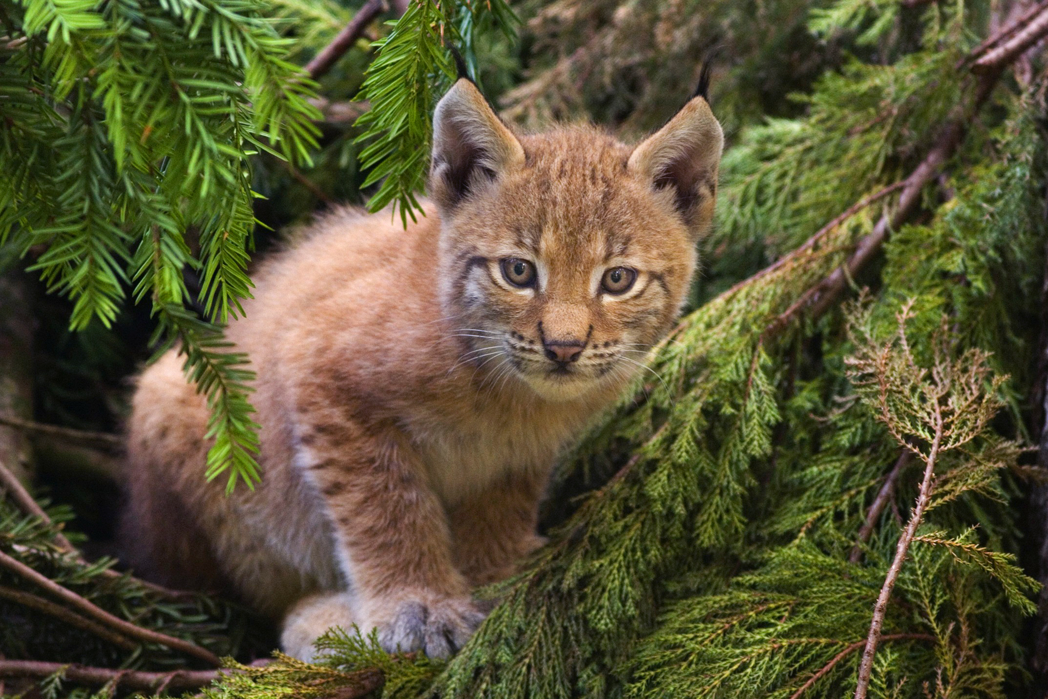
The Eurasian lynx¹⁴ is a wild cat that lives in the north of Europe and Asia. When a female lynx gives birth, she may have from 1-4 kittens. Our statistical experiment is a lynx giving birth, and the outcome is a litter of baby lynx. Baby lynx are complicated objects, but there is a simple random variable here: the number of kittens. Call this $X$. Ecologists have estimated¹⁵ the pmf for $X$ to be:

\[ \begin{array}{l|cccc} x & 1 & 2 & 3 & 4 \\ \hline p(x) & 0.18 & 0.51 & 0.27 & 0.04 \end{array} \]

In other words, the probability that a lynx mother has one kitten is 0.18, the probability that she has two kittens is 0.51, and so on. Observe that $p(0) + p(1) + p(2) + p(3) = 1$, so this is a pmf.

We can use the pmf to calculate the probability of any event defined in terms of $X$. The probability that a lynx litter has more than one kitten is: \[ P( X > 1 ) = P(X=2) + P(X=3) + P(X=4) = 0.51 + 0.27 + 0.04 = 0.82. \]

We can simulate this random variable without having to capture pregnant lynx. Recall that the R function sample has four arguments: the possible outcomes x, the sample size size to sample, whether we are sampling with replacement replace, and the probability prob associated with the possible outcomes. Here we generate values of $X$ for 30 lynx litters:

litterpmf <- c(0.18, 0.51, 0.27, 0.04)
sample(1:4, 30, replace = TRUE, prob = litterpmf)

##  [1] 1 2 2 1 2 1 1 2 3 1 3 1 1 3 3 2 1 1 3 2 2 2 3 3 3 1 2 2 3 3

With enough samples of $X$, we can approximate the probability $P(X > 1)$ as follows:

X <- sample(1:4, 10000, replace = TRUE, prob = litterpmf)
mean(X > 1)

## [1] 0.8222

In this code, the first line simulates the random variable. The code X > 1 produces a vector of TRUE and FALSE which is TRUE when the event $X > 1$ occurs. Recall that taking the mean of a TRUE/FALSE vector gives the proportion of times that vector is TRUE, which will be approximately $P(X > 1)$ here.

We can also recreate the pmf by using table to count values and then dividing by the sample size¹⁶:

table(X) / 10000

## X
##      1      2      3      4 
## 0.1778 0.5134 0.2674 0.0414

Example 3.5

Let $X$ denote the number of Heads observed when a coin is tossed three times.

In this example, we can simulate the random variable by first simulating experiment outcomes and then calculating $X$ from those. The following generates three coin flips:

coin_toss <- sample(c("H", "T"), 3, replace = TRUE)

Now we calculate how many heads were flipped, and produce one value of $X$.

sum(coin_toss == "H")

## [1] 2

Finally, we can use replicate to produce many samples of $X$:

X <- replicate(10000, {
  coin_toss <- sample(c("H", "T"), 3, replace = TRUE)
  sum(coin_toss == "H")
})
head(X, 30) # see the first 30 values of X

##  [1] 1 0 2 2 2 2 0 1 0 2 2 1 0 1 1 2 2 1 0 2 0 3 3 1 2 0 1 0 1 3

From the simulation, we can estimate the pmf using table and dividing by the number of samples:

table(X) / 10000

## X
##      0      1      2      3 
## 0.1279 0.3756 0.3743 0.1222

Instead of simulation, we could also calculate the pmf by considering the sample space, which consists of the eight equally likely outcomes HHH, HHT, HTH, HTT, THH, THT, TTH, TTT. Counting heads, we find that $X$ has the pmf:

\[ \begin{array}{l|cccc} x & 0 & 1 & 2 & 3 \\ \hline p(x) & \frac{1}{8} & \frac{3}{8} & \frac{3}{8} & \frac{1}{8} \end{array} \]

which matches the results of our simulation. Here is an alternate description of $p$ as a formula: \[ p(x) = {\binom{3}{x}} \left(\frac{1}{2}\right)^x \qquad x = 0,\ldots,3 \]

We always assume that $p$ is zero for values not mentioned; both in the table version and in the formula version.

As in the lynx example, we may simulate this random variable directly by sampling with probabilities given by the pmf. Here we sample 30 values of $X$ without “flipping” any “coins”:

sample(0:3, 30, replace = TRUE, prob = c(0.125, 0.375, 0.375, 0.125))

##  [1] 3 1 3 0 3 1 1 2 3 0 1 2 0 0 0 2 2 1 1 3 3 1 0 2 1 1 1 1 3 1

Example 3.6

Compute the probability that we observe at least one head when three coins are tossed.

Let $X$ be the number of heads. We want to compute the probability of the event $X \ge 1$. Using the pmf for $X$,

\[\begin{align*} P(1 \le X) &= P(1 \le X \le 3)\\ &=P(X = 1) + P(X = 2) + P(X = 3)\\ &= \frac{3}{8}+ \frac{3}{8} +\frac{1}{8}\\ &= \frac{7}{8} = 0.875. \end{align*}\]

We could also estimate $P(X \ge 1)$ by simulation:

X <- replicate(10000, {
  coin_toss <- sample(c("H", "T"), 3, replace = TRUE)
  sum(coin_toss == "H")
})
mean(X >= 1)

## [1] 0.8741

Example 3.7

Suppose you toss a coin until the first time you see heads. Let $X$ denote the number of tails that you see. We will see later that the pmf of $X$ is given by \[ p(x) = \left(\frac{1}{2}\right)^{x + 1} \qquad x = 0, 1, 2, 3, \ldots \] Compute $P(X = 2)$, $P(X \le 1)$, $P(X > 1)$, and the conditional probability $P(X = 2 | X > 1)$.

To compute $P(X = 2)$, we just plug in $P(X = 2) = p(2) = \left(\frac{1}{2}\right)^3 = \frac{1}{8}$.
To compute $P(X \le 1)$ we add $P(X = 0) + P(X = 1) = p(0) + p(1) = \frac{1}{2} + \frac{1}{4} = \frac{3}{4}$.
The complement of $X > 1$ is $X \le 1$, so \[ P(X > 1) = 1 - P(X \le 1) = 1 - \frac{3}{4} = \frac{1}{4}. \] Alternately, we could compute an infinite sum using the formula for the geometric series: \[ P(X > 1) = p(2) + p(3) + p(4) + \dotsb = \frac{1}{8} + \frac{1}{16} + \frac{1}{32} + \dotsb = \frac{1}{4}. \]
The formula for conditional probability gives: \[ P(X = 2 | X > 1) = \frac{P(X = 2 \cap X > 1)}{P(X > 1)} = \frac{P(X = 2)}{P(X > 1)} = \frac{1/8}{1/4} = \frac{1}{2}.\] This last answer makes sense because $X > 1$ requires the first two flips to be tails, and then there is a $\frac{1}{2}$ chance your third flip will be heads and achieve $X = 2$.

3.2 Expected value

Suppose you perform a statistical experiment repeatedly, and observe the value of a random variable $X$ each time. The average of these observations will (under most circumstances) converge to a fixed value as the number of observations becomes large. This value is the expected value of $X$, written $E[X]$.

Theorem 3.2 (Law of Large Numbers)

The mean of $n$ observations of a random variable $X$ converges to the expected value $E[X]$ as $n \to \infty$.

Another word for the expected value of $X$ is the mean of $X$.

Example 3.8

Using simulation, we determine the expected value of a die roll. Here are 30 observations and their average:

rolls <- sample(1:6, 30, replace = TRUE)
rolls

##  [1] 3 3 3 3 1 5 1 2 2 3 3 6 5 1 1 6 6 5 2 6 5 2 5 2 6 1 3 6 6 5

mean(rolls)

## [1] 3.6

The mean appears to be somewhere between 3 and 4. Using more trials gives more accuracy:

rolls <- sample(1:6, 100000, replace = TRUE)
mean(rolls)

## [1] 3.4934

Not surprisingly, the mean value is balanced halfway between 1 and 6, at 3.5.

Using the probability distribution of a random variable $X$, one can compute the expected value $E[X]$ exactly:

Definition 3.9

For a discrete random variable $X$ with pmf $p$, the expected value of $X$ is \[ E[X] = \sum_x x p(x) \] where the sum is taken over all possible values of the random variable $X$.

Example 3.10

Let $X$ be the value of a six-sided die roll. Since the probability of each outcome is $\frac{1}{6}$, we have: \[ E[X] = 1\cdot\frac{1}{6} + 2\cdot\frac{1}{6} +3\cdot\frac{1}{6} +4\cdot\frac{1}{6} +5\cdot\frac{1}{6} +6\cdot\frac{1}{6} = \frac{21}{6} = 3.5 \]

Example 3.11

Let $X$ be the number of kittens in a Eurasian lynx litter. Then \[ E[X] = 1\cdot p(1) + 2 \cdot p(2) + 3 \cdot p(3) + 4 \cdot p(4) = 0.18 + 2\cdot 0.51 + 3\cdot0.27 + 4\cdot0.04 = 2.17 \] This means that, on average, the Eurasian lynx has 2.17 kittens.

We can perform the computation of $E[X]$ using R:

litterpmf <- c(0.18, 0.51, 0.27, 0.04)
sum((1:4) * litterpmf)

## [1] 2.17

Alternatively, we may estimate $E[X]$ by simulation, using the Law of Large Numbers.

X <- sample(1:4, 10000, replace = TRUE, prob = litterpmf)
mean(X)

## [1] 2.1645

Alert 3.1

The expected value need not be a possible outcome associated with the random variable. You will never roll a 3.5, and a lynx mother will never have 2.17 kittens. The expected value describes the average of many observations.

Example 3.12

Let $X$ denote the number of heads observed when three coins are tossed. The pmf of $X$ is given by $p(x) = {\binom{3}{x}} (1/2)^x$, where $x = 0,\ldots,3$. The expected value of $X$ is

\[ E[X] = 0 \cdot \frac{1}{8} + 1 \cdot \frac{3}{8} + 2 \cdot \frac{3}{8} + 3 \cdot \frac{1}{8} = \frac{3}{2} . \]

We can check this with simulation:

X <- replicate(10000, {
  coin_toss <- sample(c("H", "T"), 3, replace = TRUE)
  sum(coin_toss == "H")
})
mean(X)

## [1] 1.4932

The answer is approximately 1.5, which is what our exact computation of $E[X]$ predicted.

Example 3.13

Consider the random variable $X$ which counts the number of tails observed before the first head when a fair coin is repeatedly tossed. The pmf of $X$ is $p(x) = 0.5^{x + 1}$ for $x = 0, 1, 2, \ldots$. Finding the expected value requires summing an infinite series, which we leave as an exercise. Instead, we proceed by simulation.

We assume (see the next paragraph for a justification) that the infrequent results of $x \ge 100$ do not impact the expected value much. This assumption needs to be checked, because it is certainly possible that low probability events which correspond to very high values of the random variable could have a large impact on the expected value. Then, we take a sample of size 10000 and follow the same steps as in the previous example.

xs <- 0:99
probs <- .5^xs
X <- sample(0:99, 10000, replace = TRUE, prob = probs)
mean(X)

## [1] 1.0172

We estimate that the expected value $E[X] \approx 1$.

To justify that we do not need to include values of $x$ bigger than 99, note that

\[\begin{align*} E[X] - \sum_{n = 0}^{99} n (1/2)^{n + 1} &= \sum_{n=100}^\infty n (1/2)^{n + 1} \\ &< \sum_{n=100}^\infty 2^{n/2 - 1} (1/2)^{n + 1}\\ &= \sum_{n = 100}^\infty 2^{-n/2}\\ &= 2^{-50} \frac{1}{2^{49}(2 - \sqrt{2})} < 10^{-14} \end{align*}\]

So, truncating the sum at $n = 99$ introduces a negligible error. The Loops in R vignette at the end of Chapter 5 shows an approach using loops that avoids truncation.

Example 3.14

We end this short section with an example of a discrete random variable that has expected value of $\infty$. Let $X$ be a random variable such that $P(X = 2^x) = 2^{-x}$ for $x = 1,2,\ldots$. We see that $\sum_{n=1}^\infty n p(n) = \sum_{n=1}^\infty 2^n 2^{-n} = \infty$. If we truncated the sum associated with $E[X]$ for this random variable at any finite point, then we would introduce a very large error!

3.3 Binomial and geometric random variables

The binomial and geometric random variables are common and useful models for many real situations. Both involve Bernoulli trials, named after the 17th century Swiss mathematician Jacob Bernoulli.

Definition 3.15

A Bernoulli trial is an experiment that can result in two outcomes, which we will denote as “success” and “failure”. The probability of a success will be denoted $p$, and the probability of failure is therefore $1-p$.

Example 3.16

The following are examples of Bernoulli trials, at least approximately.

Toss a coin. Arbitrarily define heads to be success. Then $p = 0.5$.
Shoot a free throw, in basketball. Success would naturally be making the shot, failure missing the shot. Here $p$ varies depending on who is shooting. An excellent basketball player might have $p = 0.8$.
Ask a randomly selected voter whether they support a ballot proposition. Here success would be a yes vote, failure a no vote, and $p$ is likely unknown but of interest to the person doing the polling.
Roll a die, and consider success to be rolling a six. Then $p = 1/6$.

A Bernoulli process is a sequence (finite or infinite) of repeated, identical, independent Bernoulli trials. Repeatedly tossing a coin is a Bernoulli process. Repeatedly trying to roll a six is a Bernoulli process. Is repeated free throw shooting a Bernoulli process? There are two reasons that it might not be. First, if the person shooting is a beginner, then they would presumably get better with practice. That would mean that the probability of a success is not the same for each trial (especially if the number of trials is large), and the process would not be Bernoulli. Second, there is the more subtle question of whether free throws are independent. Does a free throw shooter get “hot” and become more likely to make the shot following a success? There is no way to know for sure, although research¹⁷ suggests that repeated free throws are independent and that modeling free throws of experienced basketball players with a Bernoulli process is reasonable.

This section discusses two discrete random variables coming from a Bernoulli process: the binomial random variable which counts the number of successes in a fixed number of trials, and the geometric random variable, which counts the number of trials before the first success.

3.3.1 Binomial

Definition 3.17

A random variable $X$ is said to be a binomial random variable with parameters $n$ and $p$ if \[ P(X = x) = {\binom{n}{x}} p^x (1 - p)^{n - x}\qquad x = 0, 1, \ldots, n. \] We will sometimes write $X \sim \text{Binom}(n,p)$

The most important example of a binomial random variable comes from counting the number of successes in a Bernoulli process of length $n$. In other words, if $X$ counts the number of successes in $n$ independent and identically distributed Bernoulli trials, each with probability of success $p$, then $X \sim \text{Binom}(n, p)$. Indeed, many texts define binomial random variables in this manner, and we will use this alternative definition of a binomial random variable whenever it is convenient for us to do so.

One way to obtain a Bernoulli process is to sample with replacement from a population. If an urn contains 5 white balls and 5 red balls, and you count drawing a red ball as a “success”, then repeatedly drawing balls will be a Bernoulli process as long as you replace the ball back in the urn after you draw it. When sampling from a large population, we can sample without replacement and the resulting count of successes will be approximately binomial.

Example 3.18

Let $X$ denote the number of heads observed when three coins are tossed. Then $X \sim \text{Binom}(3,0.5)$ is a binomial random variable. Here $n = 3$ because there are three independent Bernoulli trials, and $p = 0.5$ because each coin has probability $0.5$ of heads.

Theorem 3.3

If $X$ counts the number of successes in $n$ independent and identically distributed Bernoulli trials, each with probability of success $p$, then $X \sim \text{Binom}(n, p)$.

Proof:

There are $n$ trials. There are $\binom{n}{x}$ ways to choose $x$ of these $n$ trials as the successful trials. For each of these ways, $p^x(1-p)^{n-x}$ is the probability of having $x$ successes in the chosen spots and $n-x$ failures in the not chosen spots.

Remark

The binomial theorem says that: \[ (a + b)^n = a^n + {\binom{n}{1}}a^{n-1}b^1 + {\binom{n}{2}}a^{n-2}b^2 + \dotsb + {\binom{n}{n-1}}a^1 b^{n-1} + b^n \] Substituting $a = p$ and $b = 1-p$, the left hand side becomes $(p + 1-p)^n = 1^n = 1$, and so: \[\begin{align} 1 &= p^n + {\binom{n}{1}}p^{n-1}(1-p)^1 + {\binom{n}{2}}p^{n-2}(1-p)^2 + \dotsb + {\binom{n}{n-1}}p^1 (1-p)^{n-1} + (1-p)^n\\ &= P(X = n) + P(X = n-1) + P(X = n-2) + \dotsb + P(X = 1) + P(X = 0) \end{align}\] Which shows that the pmf for the binomial distribution does sum to 1, as it must.

In R, the function dbinom provides the pmf of the binomial distribution:

dbinom(x, size = n, prob = p) gives $P(X = x)$ for $X \sim \text{Binom}(n,p)$. If we provide a vector of values for x, and a single value of size and prob, then dbinom will compute $P(X = x)$ for all of the values in x. The idiom sum(dbinom(vec, size, prob)) will be used below, with vec containing distinct values, to compute the probability that $X$ is in the set described by vec. This is a useful idiom for all of the discrete random variables.

Example 3.19

For $X$ the number of heads when three coins are tossed, the pmf is $P(X = x) = \begin{cases} 1/8 & x = 0,3\\3/8 & x = 1,2 \end{cases}$.

Computing with R,

x <- 0:3
dbinom(x, size = 3, prob = 0.5)

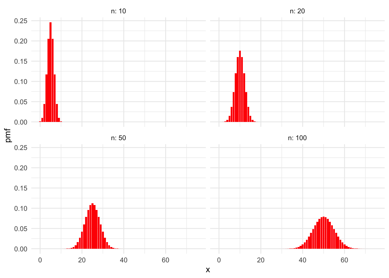
## [1] 0.125 0.375 0.375 0.125

Here are some sample plots of the pmf of a binomial rv for various values of $n$ and $p= .5$.

Here are some with $n = 100$ and various $p$.

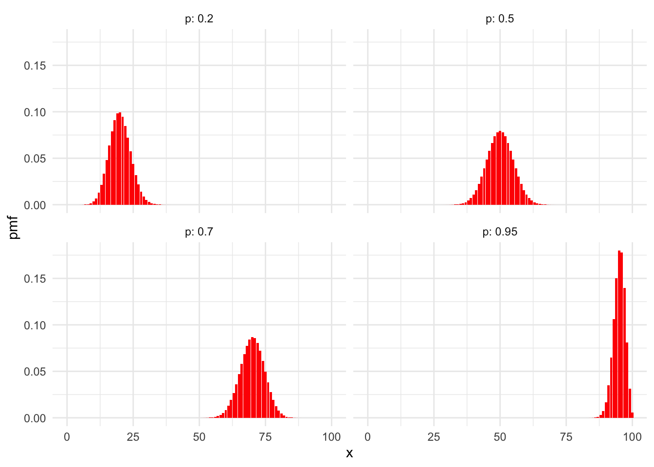
In these plots of binomial pmfs, the distributions are roughly balanced around a peak. The balancing point is the expected value of the random variable, which for binomial rvs is quite intuitive:

Theorem 3.4

Let $X$ be a binomial random variable with $n$ trials and probability of success $p$. Then \[ E[X] = np \]

We will see a simple proof of this once we talk about the expected value of the sum of random variables. Here is a proof using the pmf and the definition of expected value directly.

Proof:

The binomial theorem says that: \[ (a + b)^n = a^n + {\binom{n}{1}}a^{n-1}b^1 + {\binom{n}{2}}a^{n-2}b^2 + \dotsb + {\binom{n}{n-1}}a^1 b^{n-1} + b^n \] Take the derivative of both sides with respect to $a$: \[ n(a + b)^{n-1} = na^{n-1} + (n-1){\binom{n}{1}}a^{n-2}b^1 + (n-2){\binom{n}{2}}a^{n-3}b^2 + \dotsb + 1{\binom{n}{n-1}}a^0 b^{n-1} + 0 \] Multiply both sides by $a$: \[ an(a + b)^{n-1} = na^{n} + (n-1){\binom{n}{1}}a^{n-1}b^1 + (n-2){\binom{n}{2}}a^{n-2}b^2 + \dotsb + 1{\binom{n}{n-1}}a^1 b^{n-1} + 0\] Finally, substitute $a = p$, $b = 1-p$, and note that $a + b = 1$: \[ pn = np^{n} + (n-1){\binom{n}{1}}p^{n-1}(1-p)^1 + (n-2){\binom{n}{2}}p^{n-2}(1-p)^2 + \dotsb + 1{\binom{n}{n-1}}p^1 (1-p)^{n-1} + 0(1-p)^n \] or \[ pn = \sum_{x = 0}^{n} x {\binom{n}{x}}p^x(1-p)^{n-x} = E[X] \] Since for $X \sim \text{Binom}(n,p)$, the pmf is given by $P(X = x) = {\binom{n}{x}}p^{x}(1-p)^{n-x}$

Example 3.20

Suppose 100 dice are thrown. What is the expected number of sixes? What is the probability of observing 10 or fewer sixes?

We assume that the results of the dice are independent and that the probability of rolling a six is $p = 1/6$. The random variable $X$ is the number of sixes observed, and $X \sim \text{Binom}(100,1/6)$.

Then $E[X] = 100 \cdot \frac{1}{6} \approx 16.67$. That is, we expect 1/6 of the 100 rolls to be a six.

The probability of observing 10 or fewer sixes is \[ P(X \le 10) = \sum_{j=0}^{10} P(X = j) = \sum_{j=0}^{10} {\binom{100}{j}}(1/6)^j(5/6)^{100-j} \approx 0.0427. \] In R,

sum(dbinom(0:10, 100, 1 / 6))

## [1] 0.04269568

R also provides the function pbinom, which is the cumulative sum of the pmf. The cumulative sum of a pmf is important enough that it gets its own name: the cumulative distribution function. We will say more about the cumulative distribution function in general in Section 4.1.

pbinom(x, size = n, prob = p) gives $P(X \leq x)$ for $X \sim \text{Binom}(n,p)$.

In the previous example, we could compute $P(X \le 10)$ as

pbinom(10, 100, 1 / 6)

## [1] 0.04269568

Example 3.21

Suppose Alice and Bob are running for office, and 46% of all voters prefer Alice. A poll randomly selects 300 voters from a large population and asks their preference. What is the expected number of voters who will report a preference for Alice? What is the probability that the poll results suggest Alice will win?

Let “success” be a preference for Alice, and $X$ be the random variable equal to the number of polled voters who prefer Alice. It is reasonable to assume that $X \sim \text{Binom}(300,0.46)$ as long as our sample of 300 voters is a small portion of the population of all voters.

We expect that $0.46 \cdot 300 = 138$ of the 300 voters will report a preference for Alice.

For the poll results to show Alice in the lead, we need $X > 150$. To compute $P(X > 150)$, we use $P(X > 150) = 1 - P(X \leq 150)$ and then

1 - pbinom(150, 300, 0.46)

## [1] 0.07398045

There is about a 7.4% chance the poll will show Alice in the lead, despite her imminent defeat.

R provides the function rbinom to simulate binomial random variables. The first argument to rbinom is the number of random values to simulate, and the next arguments are size = n and prob = p. Here are 15 simulations of the Alice vs. Bob poll:

rbinom(15, size = 300, prob = 0.46)

##  [1] 132 116 129 139 165 137 138 142 134 140 140 134 134 126 149

In this series of simulated polls, Alice appears to be losing in all except the fifth poll where she was preferred by $165/300 = 55\%$ of the selected voters.

We can compute $P(X > 150)$ by simulation

X <- rbinom(10000, 300, 0.46)
mean(X > 150)

## [1] 0.0714

which is close to our theoretical result that Alice should appear to be winning 7.4% of the time.

Finally, we can estimate the expected number of people in our poll who say they will vote for Alice and compare that to the value of 138 that we calculated above.

mean(X) # estimate of expected value

## [1] 137.9337

3.3.2 Geometric

Definition 3.22

A random variable $X$ is said to be a geometric random variable with parameter $p$ if \[ P(X = x) = (1 - p)^{x} p, \qquad x = 0, 1,2, \ldots \]

Theorem 3.5

Let $X$ be the random variable that counts the number of failures before the first success in a Bernoulli process with probability of success $p$. Then $X$ is a geometric random variable.

Proof:

The only way to achieve $X = x$ is to have the first $x$ trials result in failure and the next trial result in success. Each failure happens with probability $1-p$, and the final success happens with probability $p$. Since the trials are independent, we multiply $1-p$ a total of $x$ times, and then multiply by $p$.

As a check, we show that the geometric pmf does sum to one. This requires summing an infinite geometric series: \[ \sum_{x=0}^{\infty} p(1-p)^x = p \sum_{x=0}^\infty (1-p)^x = p \frac{1}{1-(1-p)} = 1 \]

Alert 3.2

We defined the geometric random variable $X$ so that it is compatible with functions built in to R. Some sources let $Y$ be the number of trials required for the first success, and call $Y$ geometric. In that case $Y = X + 1$, as the final success counts as one additional trial.

The functions dgeom, pgeom and rgeom are available for working with a geometric random variable $X \sim \text{Geom}(p)$:

dgeom(x,p) is the pmf, and gives $P(X = x)$
pgeom(x,p) gives $P(X \leq x)$
rgeom(N,p) simulates $N$ random values of $X$.

Example 3.23

A die is tossed until the first 6 occurs. What is the probability that it takes 4 or more tosses?

We define success as a roll of six, and let $X$ be the number of failures before the first success. Then $X \sim \text{Geom}(1/6)$, a geometric random variable with probability of success $1/6$.

Taking 4 or more tosses corresponds to the event $X \geq 3$. Theoretically, \[ P(X \ge 3) = \sum_{x=3}^\infty P(X = x) = \sum_{x=3}^\infty \frac{1}{6}\cdot\left(\frac{5}{6}\right)^x = \frac{125}{216} \approx 0.58. \] We cannot perform the infinite sum with dgeom, but we can come close by summing to a large value of $x$:

sum(dgeom(3:1000, 1 / 6))

## [1] 0.5787037

Another approach is to apply rules of probability to see that $P(X \ge 3) = 1 - P(X < 3)$ Since $X$ is discrete, $X < 3$ and $X \leq 2$ are the same event. Then $P(X \ge 3) = 1 - P(X \le 2)$:

1 - sum(dgeom(0:2, 1 / 6))

## [1] 0.5787037

Rather than summing the pmf, we may use pgeom:

1 - pgeom(2, 1 / 6)

## [1] 0.5787037

The function pgeom has an option lower.tail=FALSE which makes it compute $P(X > x)$ rather than $P(X \le x)$, leading to maybe the most concise method:

pgeom(2, 1 / 6, lower.tail = FALSE)

## [1] 0.5787037

Finally, we can use simulation to approximate the result:

X <- rgeom(10000, 1 / 6)
mean(X >= 3)

## [1] 0.581

All of these show there is about a 0.58 probability that it will take four or more tosses to roll a six.

Here are some plots of geometric pmfs with various $p$.

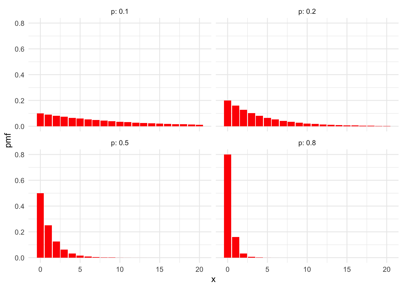
Observe that for smaller $p$, we see that $X$ is likely to be larger. The lower the probability of success, the more failures we expect before our first success.

Theorem 3.6

Let $X$ be a geometric random variable with probability of success $p$. Then \[ E[X] = \frac{(1-p)}{p} \]

Proof:

Let $X$ be a geometric rv with success probability $p$. Let $q = 1-p$ be the failure probability. We must compute $E[X] = \sum_{x = 0}^\infty x pq^x$. Begin with a geometric series in $q$: \[ \sum_{x = 0}^\infty q^x = \frac{1}{1-q} \] Take the derivative of both sides with respect to $q$: \[ \sum_{x = 0}^\infty xq^{x-1} = \frac{1}{(1-q)^2} \] Multiply both sides by $pq$: \[ \sum_{x = 0}^\infty xpq^x = \frac{pq}{(1-q)^2} \] Replace $1-q$ with $p$ and we have shown: \[ E[X] = \frac{q}{p} = \frac{1-p}{p} \]

Example 3.24

Roll a die until a six is tossed. What is the expected number of rolls?

The expected number of failures is given by $X \sim \text{Geom}(1/6)$, and so we expect $\frac{5/6}{1/6} = 5$ failures before the first success. Since the number of total rolls is one more than the number of failures, we expect 6 rolls, on average, to get a six.

Example 3.25

Professional basketball player Steve Nash was a 90% free throw shooter over his career. If Steve Nash starts shooting free throws, how many would he expect to make before missing one? What is the probability that he could make 20 in a row?

Let $X$ be the random variable which counts the number of free throws Steve Nash makes before missing one. We model a Steve Nash free throw as a Bernoulli trial, but we choose “success” to be a missed free throw, so that $p = 0.1$ and $X \sim \text{Geom}(0.1)$. The expected number of “failures” is $E[X] = \frac{0.9}{0.1} = 9$, which means we expect Steve to make 9 free throws before missing one.

To make 20 in a row requires $X \ge 20$. Using $P(X \ge 20) = 1 - P(X \le 19)$,

1 - pgeom(19, 0.1)

## [1] 0.1215767

we see that Steve Nash could run off 20 (or more) free throws in a row about 12% of the times he wants to try.

3.4 Functions of a random variable

Recall that a random variable $X$ is a function from the sample space $S$ to $\mathbb{R}$. Given a function $g : \mathbb{R} \to \mathbb{R},$ we can form the random variable $g \circ X$, usually written $g(X)$.

For example, the mean number of births per day in the United States is about 10300. Suppose we pick a day in February and observe $X$ the number of births on that day. We might be more interested in the deviation from the mean $X - \mu$ or the absolute deviation from the mean $|X - \mu|$ of the measurement than we are in $X$, the value of the measurement. The values $X - \mu$ and $|X - \mu|$ are examples of functions of a random variable.

As another example, if $X$ is the value from a six-sided die roll and $g(x) = x^2$, then $g(X) = X^2$ is the value of a single six-sided die roll, squared. Here $X^2$ can take the values $1, 4, 9, 16, 25, 36$, all equally likely.

The probability mass function of $g(X)$ can be computed as follows. For each $y$, the probability that $g(X) = y$ is given by $\sum p(x)$, where the sum is over all values of $x$ such that $g(x) = y$.

Example 3.26

Let $X$ be the value when a six-sided die is rolled and let $g(X) = X^2$. The probability mass function of $g(X)$ is given by

\[ \begin{array}{l|cccccc} x & 1 & 4 & 9 & 16 & 25 & 36 \\ \hline p(x) & 1/6 & 1/6 & 1/6 & 1/6 & 1/6 & 1/6 \end{array} \]

This is because for each value of $y$, there is exactly one $x$ with positive probability for which $g(x) = y$.

Example 3.27

Let $X$ be the value when a six-sided die is rolled and let $g(X) = |X - 3.5|$ be the absolute deviation from the expected value.¹⁸ The probability that $g(X) = .5$ is 2/6 because $g(4) = g(3) = 0.5$, and $p(4) + p(3) = 2/6$. The full probability mass function of $g(X)$ is given by

\[ \begin{array}{l|ccc} x & 0.5 & 1.5 & 2.5 \\ \hline p(x) & 1/3 & 1/3 & 1/3 \end{array} \]

Note that we could then find the expected value of $g(X)$ by applying the definition of expected value to the probability mass function of $g(X)$. It is usually easier, however, to apply the following theorem.

Theorem 3.7

Let $X$ be a discrete random variable with probability mass function $p$, and let $g$ be a function. Then, \[ E\left[g(X)\right] = \sum g(x) p(x). \]

Example 3.28

Let $X$ be the value of a six-sided die roll. Then whether we use the pmf calculated in Example 3.26 or Theorem 3.7, we get that \[ E[X^2] = 1^2\cdot 1/6 + 2^2\cdot 1/6 + 3^2\cdot 1/6 + 4^2\cdot 1/6 + 5^2\cdot 1/6 + 6^2\cdot 1/6 = 91/6 \approx 15.17\] Computing with simulation is straightforward:

X <- sample(1:6, 10000, replace = TRUE)
mean(X^2)

## [1] 15.072

Example 3.29

Let $X$ be the number of heads observed when a fair coin is tossed three times. Compute the expected value of $(X-1.5)^2$. Since $X$ a binomial random variable with $n = 3$ and $p = 1/2$, it has pmf $p(x) = {\binom{3}{x}} (.5)^3$ for $x = 0,1,2,3$. We compute \[ \begin{split} E[(X-1.5)^2] &= \sum_{x=0}^3(x-1.5)^2p(x)\\ &= (0-1.5)^2\cdot 0.125 + (1-1.5)^2 \cdot 0.375 + (2-1.5)^2 \cdot 0.375 + (3-1.5)^2 \cdot 0.125\\ &= 0.75 \end{split} \] Since dbinom gives the pdf for binomial rvs, we can perform this exact computation in R:

x <- 0:3
sum((x - 1.5)^2 * dbinom(x, 3, 0.5))

## [1] 0.75

We conclude this section with two simple but important observations about expected values. First, that expected value is linear. Second, that the expected value of a constant is that constant. Stated precisely:

Theorem 3.8

For random variables $X$ and $Y$, and constants $a$, $b$, and $c$:

$E[aX + bY] = aE[X] + bE[Y]$
$E[c] = c$

The proofs follow from the definition of expected value and the linearity of summation. With these theorems in hand, we can provide a much simpler proof for the formula of the expected value of a binomial random variable.

Let $X \sim \text{Binom}(n, p)$. Then $X$ is the number of successes in $n$ Bernoulli trials, each with probability $p$. Let $X_1, \ldots, X_n$ be independent Bernoulli random variables with probability of success $p$. That is, $P(X_i = 1) = p$ and $P(X_i = 0) = 1 - p$. It follows that $X = \sum_{i = 1}^n X_i$. Therefore,

\[\begin{align*} E[X] &= E[\sum_{i = 1}^n X_i]\\ &= \sum_{i = 1}^n E[X_i] = \sum_{i = 1}^n p = np. \end{align*}\]

3.5 Variance, standard deviation and independence

The variance of a random variable measures the spread of the variable around its expected value. Random variables with large variance can be quite far from their expected values, while rvs with small variance stay near their expected value. The standard deviation is simply the square root of the variance. The standard deviation also measures spread, but in more natural units which match the units of the random variable itself.

Definition 3.30

Let $X$ be a random variable with expected value $\mu = E[X]$. The variance of $X$ is defined as \[ \text{Var}(X) = E[(X - \mu)^2] \] The standard deviation of $X$ is written $\sigma(X)$ and is the square root of the variance: \[ \sigma(X) = \sqrt{\text{Var}(X)} \]

Note that the variance of an rv is always positive (in the French sense¹⁹), as it is the sum of a positive function.

The next theorem gives a formula for the variance that is often easier than the definition when performing computations.

Theorem 3.9

${\rm Var}(X) = E[X^2] - E[X]^2$

Proof:

Applying linearity of expected values (Theorem 3.8) to the definition of variance yields: \[ \begin{split} E[(X - \mu)^2] &= E[X^2 - 2\mu X + \mu^2]\\ &= E[X^2] - 2\mu E[X] + \mu^2 = E[X^2] - 2\mu^2 + \mu^2\\ &= E[X^2] - \mu^2, \end{split} \] as desired.

Example 3.31

Let $X \sim \text{Binom}(3,0.5)$. Here $\mu = E[X] = 1.5$. In Example 3.29, we saw that $E[(X-1.5)^2] = 0.75$. Then $\text{Var}(X) = 0.75$ and the standard deviation is $\sigma(X) = \sqrt{0.75} \approx 0.866$. We can check both of these using simulation and the built in R functions var and sd:

X <- rbinom(10000, 3, 0.5)
var(X)

## [1] 0.7707854

sd(X)

## [1] 0.8779438

For many distributions, most of the values will lie within one standard deviation of the mean, i.e. within the spread shown in the example pictures. Almost all of the values will lie within 2 standard deviations of the mean. What do we mean by “almost all”? Well, 85% would be almost all. 15% would not be almost all. This is a very vague rule of thumb. Chebychev’s Theorem is a more precise statement. It says in particular that the probability of being more than 2 standard deviations away from the mean is at most 25%.

Sometimes, you know that the data you collect will likely fall in a certain range of values. For example, if you are measuring the height in inches of 100 randomly selected adult males, you would be able to guess that your data will very likely lie in the interval 60-84. You can get a rough estimate of the standard deviation by taking the expected range of values and dividing by 6; in this case it would be 24/6 = 4. Here, we are using the heuristic that it is very rare for data to fall more than three standard deviations from the mean. This can be useful as a quick check on your computations.

3.5.1 Independent random variables

Unlike expected value, variance and standard deviation are not linear. However, variance and standard deviation do have scaling properties, and variance does distribute over sums in the special case of independent random variables.

We say that two random variables, $X$ and $Y$, are independent if knowledge of the outcome of $X$ does not give probabilistic information about the outcome of $Y$ and vice versa. As an example, let $X$ be the amount of rain (in inches) recorded at Lambert Airport on a randomly selected day in 2017, and let $Y$ be the height of a randomly selected person in Botswana. It is difficult to imagine that knowing the value of one of these random variables could give information about the other one, and it is reasonable to assume that the rvs are independent. On the other hand, if $X$ and $Y$ are the height and weight of a randomly selected person in Botswana, then knowledge of one variable could well give probabilistic information about the other. For example, if you know a person is 72 inches tall, it is unlikely that they weigh 100 pounds.

We would like to formalize that notion with conditional probability. The natural statement is that for any $E, F$ subsets of ${\mathbb R}$, the conditional probability $P(X\in E|Y\in F)$ is equal to $P(X \in E)$. There are several issues with formalizing the notion of independence that way, so we give a definition that is somewhat further removed from the intuition.

The definition mirrors the multiplication rule for independent events.

Definition 3.32

Suppose $X$ and $Y$ are random variables:

$X$ and $Y$ are independent $\iff$ For all $x$ and $y$, $P(X \le x, Y \le y) = P(X \le x) P(Y \le y)$.

For discrete random variables, this is equivalent to saying that $P(X = x, Y = y) = P(X = x)P(Y = y)$ for all $x$ and $y$.

For our purposes, we will often be assuming that random variables are independent.

Theorem 3.10

Let $X$ be a rv and $c$ a constant. Then \[ \begin{aligned} \text{Var}(cX) &= c^2\text{Var}(X)\\ \sigma(cX) &= c \sigma(X) \end{aligned} \]
Let $X$ and $Y$ be independent random variables. Then \[ {\rm Var}(aX + bY) = a^2 {\rm Var}(X) + b^2 {\rm Var}(Y) \]

Proof:

We prove part 1 here, and verify part 2 through simulation in Exercise 4.13. \[\begin{align*} {\rm Var}(cX) =& E[(cX)^2] - E[cX]^2 = c^2E[X^2] - (cE[X])^2\\ =&c^2\bigl(E[X^2] - E[X]^2) = c^2{\rm Var}(X) \end{align*}\]

Alert 3.3

Theorem 3.10 part 2 is only true when $X$ and $Y$ are independent.
If $X$ and $Y$ are independent, then ${\rm Var}(X - Y) = {\rm Var}(X) + {\rm Var}(Y)$.

Example 3.33 (The variance of a binomial random variable)

Let $X \sim \text{Binom}(n, p)$. We have seen that $X = \sum_{i = 1}^n X_i$, where $X_i$ are independent Bernoulli random variables. Therefore,

\[\begin{align*} {\text {Var}}(X) &= {\text {Var}}(\sum_{i = 1}^n X_i)\\ &= \sum_{i = 1}^n {\text {Var}}(X_i) \\ &= \sum_{i = 1}^n p(1 - p) = np(1-p) \end{align*}\] where we have used that the variance of a Bernoulli random variable is $p(1- p)$. Indeed, $E[X_i^2] -E[X_i]^2 = p - p^2 = p(1 - p)$.

3.6 Poisson, negative binomial and hypergeometric

In this section, we discuss other commonly occurring special types of discrete random variables.

3.6.1 Poisson

A Poisson process models events that happen at random times. For example, radioactive decay is a Poisson process, where each emission of a radioactive particle is an event. Other examples modeled by Poisson process are meteor strikes on the surface of the moon, customers arriving at a store, hits on a web page, and car accidents on a given stretch of highway.

Figure 3.1

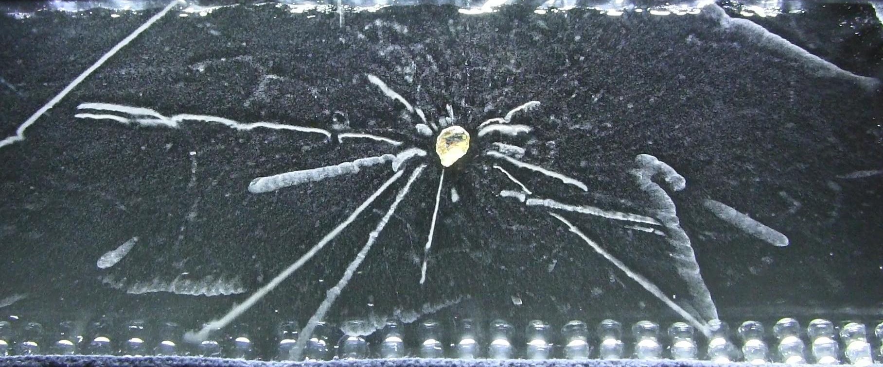
Figure 3.1: Radioactivity of a Thorite mineral seen in a cloud chamber. (Photo credit: Julien Simon)

In this section, we will discuss one natural random variable attached to a Poisson process: the Poisson random variable . We will see another, the exponential random variable , in Section 4.4.2. The Poisson random variable is discrete, and can be used to model the number of events that happen in a fixed time period. The exponential random variable models the time between events.

We begin by defining a Poisson process. Suppose events occur spread over time. The events form a Poisson process if they satisfy the following assumptions:

Assumptions 3.1 (for a Poisson process)

The probability of an event occurring in a time interval $[a,b]$ depends only on the length of the interval $[a,b]$.
If $[a,b]$ and $[c,d]$ are disjoint time intervals, then the probability that an event occurs in $[a,b]$ is independent of whether an event occurs in $[c,d]$. (That is, knowing that an event occurred in $[a,b]$ does not change the probability that an event occurs in $[c,d]$.)
Two events cannot happen at the same time. (Formally, we need to say something about the probability that two or more events happens in the interval $[a, a + h]$ as $h\to 0$.)
The probability of an event occurring in a time interval $[a,a + h]$ is roughly $\lambda h$, for some constant $\lambda$.

Property 4 says that events occur at a certain rate, which is denoted by $\lambda$.

Definition 3.34

The random variable $X$ is said to be a Poisson random variable with rate $\lambda$ if the pmf of $X$ is given by \[ p(x) = e^{-\lambda} \frac{\lambda^x}{x!} \qquad x = 0, 1, 2, \ldots \] The parameter $\lambda$ is required to be larger than 0. We write $X \sim \text{Pois}(\lambda)$.

Theorem 3.11

Let $X$ be the random variable that counts the number of occurrences in a Poisson process with rate $\lambda$ over one unit of time. Then $X$ is a Poisson random variable with rate $\lambda$.

Proof: (heuristic)

We have not stated Assumption 3.1.4 precisely enough for a formal proof, so this is only a heuristic argument.

Suppose we break up the time interval from 0 to 1 into $n$ pieces of equal length. Let $X_i$ be the number of events that happen in the $i$th interval. When $n$ is big, $(X_i)_{i = 1}^n$ is approximately a sequence of $n$ Bernoulli trials, each with probability of success $\lambda/n$. Therefore, if we let $Y_n$ be a binomial random variable with $n$ trials and probability of success $\lambda/n$, we have:

\[\begin{align*} P(X = x) &= P(\sum_{i = 1}^n X_i = x)\\ &\approx P(Y_n = x)\\ &= {\binom{n}{x}} (\lambda/n)^x (1 - \lambda/n)^{(n - x)} \\ &\approx \frac{n^x}{x!} \frac{1}{n^x} \lambda^x (1 - \lambda/n)^n\\ &\to \frac{\lambda^x}{x!}{e^{-\lambda}} \qquad {\text {as}} \ n\to \infty \end{align*}\]

The key to defining the Poisson process formally correctly is to ensure that the above computation is mathematically justified.

We leave the proof that $\sum_x p(x) = 1$ as Exercise 3.31, along with the proof of the following Theorem.

Theorem 3.12

The mean and variance of a Poisson random variable are both $\lambda$.

Though the proof of the mean and variance of a Poisson is an exercise, we can also give a heuristic argument. From above, a Poisson with rate $\lambda$ is approximately a Binomial rv $Y_n$ with $n$ trials and probability of success $\lambda/n$ when $n$ is large. The mean of $Y_n$ is $n \times \lambda/n = \lambda$, and the variance is $n (\lambda/n)(1 - \lambda/n) \to \lambda$ as $n\to\infty$.

Here some plots of Poisson pmfs with various means $\lambda$.

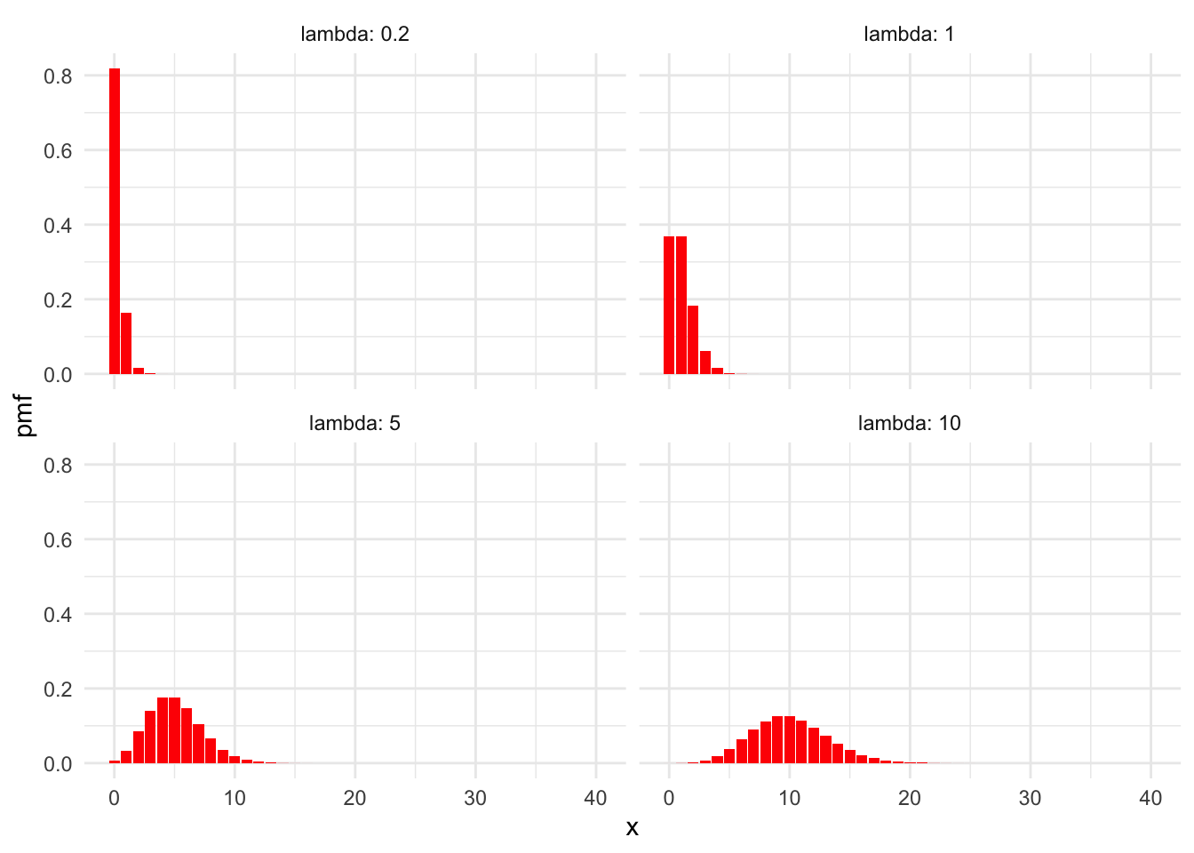
Observe in the plots that larger values of $\lambda$ correspond to more spread-out distributions, since the standard deviation of a Poisson rv is $\sqrt{\lambda}$. Also, for larger values of $\lambda$, the Poisson distribution becomes approximately normal.

Example 3.35

The Taurids meteor shower is visible on clear nights in the Fall and can have visible meteor rates around five per hour. What is the probability that a viewer will observe exactly eight meteors in two hours?

We let $X$ be the number of observed meteors in two hours, and model $X \sim \text{Pois}(10)$, since we expect $\lambda = 10$ meteors in our two hour time period. Computing exactly, \[ P(X = 8) = \frac{10^8}{8!}e^{-10} \approx 0.1126.\]

Using R, and the pdf dpois:

dpois(8, 10)

## [1] 0.112599

Or, by simulation with rpois:

meteors <- rpois(10000, 10)
mean(meteors == 8)

## [1] 0.1081

We find that the probability of seeing exactly 8 meteors is about 0.11.

Example 3.36

Suppose a typist makes typos at a rate of 3 typos per 10 pages. What is the probability that they will make at most one typo on a five page document?

We let $X$ be the number of typos in a five page document. Assume that typos follow the properties of a Poisson rv. It is not clear that they follow it exactly. For example, if the typist has just made a mistake, it is possible that their fingers are no longer on home position, which means another mistake is likely soon after. This would violate the independence property (2) of a Poisson process. Nevertheless, modeling $X$ as a Poisson rv is reasonable.

The rate at which typos occur per five pages is 1.5, so we use $\lambda = 1.5$. Then we can compute $P(X \leq 1) = \text{ppois}(1,1.5)=0.5578$. The typist has a 55.78% chance of making at most one typo on a five page document.

3.6.2 Negative binomial

Suppose you repeatedly roll a fair die. What is the probability of getting exactly 14 non-sixes before getting your second 6?

As you can see, this is an example of repeated Bernoulli trials with $p = 1/6$, but it isn’t exactly geometric because we are waiting for the second success. This is an example of a negative binomial random variable.

Definition 3.37

Suppose that we observe a sequence of Bernoulli trials with probability of success $p$. If $X$ denotes the number of failures before the $n$th success, then $X$ is a negative binomial random variable with parameters $n$ and $p$. The probability mass function of $X$ is given by

\[ p(x) = \binom{x + n - 1}{x} p^n (1 - p)^x, \qquad x = 0,1,2\ldots \]

The mean of a negative binomial is $n p/(1 - p)$, and the variance is $n p /(1 - p)^2$. The root R function to use with negative binomials is nbinom, so dnbinom is how we can compute values in R. The function dnbinom uses prob for $p$ and size for $n$ in our formula.

Example 3.38

Suppose you repeatedly roll a fair die. What is the probability of getting exactly 14 non-sixes before getting your second 6?

dnbinom(x = 14, size = 2, prob = 1 / 6)

## [1] 0.03245274

Note that when size = 1, negative binomial is exactly a geometric random variable, e.g.

dnbinom(x = 14, size = 1, prob = 1 / 6)

## [1] 0.01298109

dgeom(14, prob = 1 / 6)

## [1] 0.01298109

3.6.3 Hypergeometric

Consider the experiment which consists of sampling without replacement from a population that is partitioned into two subgroups - one subgroup is labeled a “success” and one subgroup is labeled a “failure”. The random variable that counts the number of successes in the sample is an example of a hypergeometric random variable.

To make things concrete, we suppose that we have $m$ successes and $n$ failures. We take a sample of size $k$ (without replacement) and we let $X$ denote the number of successes. Then \[ P(X = x) = \frac{\binom{m}{x} {\binom{n}{k - x}} }{\binom{m + n}{k}} \] We also have \[ E[X] = k (\frac{m}{m + n}) \] which is easy to remember because $k$ is the number of samples taken, and the probability of a success on any one sample (with no knowledge of the other samples) is $\frac {m}{m + n}$. The variance is similar to the variance of a binomial as well, \[ V(X) = k \frac{m}{m+n} \frac {n}{m+n} \frac {m + n - k}{m + n - 1} \] but we have the “fudge factor” of $\frac {m + n - k}{m + n - 1}$, which means the variance of a hypergeometric is less than that of a binomial. In particular, when $m + n = k$, the variance of $X$ is 0. Why?

When $m + n$ is much larger than $k$, we will approximate a hypergeometric random variable with a binomial random variable with parameters $n = m + n$ and $p = \frac {m}{m + n}$. Finally, the R root for hypergeometric computations is hyper. In particular, we have the following example:

Example 3.39

15 US citizens and 20 non-US citizens pass through a security line at an airport. Ten are randomly selected for further screening. What is the probability that 2 or fewer of the selected passengers are US citizens?

In this case, $m = 15$, $n = 20$, and $k = 10$. We are looking for $P(X \le 2)$, so

sum(dhyper(x = 0:2, m = 15, n = 20, k = 10))

## [1] 0.08677992

You can find a summary of the discrete random variables together with their R commands in Section 4.5.

Vignette: An RMarkdown primer

RStudio has included a method for making higher quality documents from a combination of R code and some basic markdown formatting, which is called R Markdown. In fact, this book itself was written in an extension of RMarkdown called bookdown.

For students reading this book, writing your homework in RMarkdown will allow you to have reproducible results. It is much more efficient than creating plots in R and copy/pasting into Word or some other document. Professionals may want to write reports in RMarkdown. This chapter gives the basics, with a leaning toward homework assignments.

In order to create an R Markdown file, inside RStudio you click on File, then New File and R Markdown. You will be prompted to enter a Title and an Author. For now, leave the Default Output Format as .html and leave the Document icon highlighted. When you have entered an acceptable title and author, click OK and a new tab in the Source pane should open up. (That is the top left pane in RStudio.) The very first thing that we would do is click on the Knit button right above the source panel. It should knit the document and give you a nice-ish looking document. Our goal in this vignette is to get you started making nicer looking homework and other documents in RMarkdown. For further information, see Xie, Allaire and Grolemund’s book.²⁰

You should see something that looks like this, with some more things underneath.

---
title: “Untitled”
author: “Darrin Speegle”
date: “1/20/2021”
output: html_document
---

This part of the code is the YAML (YAML Ain’t Markup Language). Next is a bit of code that starts like this. You don’t have to change that, but you might experiment with the tufte style. You will need to install the tufte package in order to do this, and change your YAML to look like this.

---
title: "Homework 1"
author: "Darrin Speegle"
date: "1/20/2021"
output:
  tufte::tufte_handout: default
  tufte::tufte_html: default
---

```{r setup, include=FALSE}
knitr::opts_chunk$set(echo = TRUE, 
                      message = FALSE, 
                      warning = FALSE, 
                      fig.width = 4, 
                      fig.height = 4, 
                      fig.margin = TRUE)
```

One benefit of using the tufte package is that in order for the document to look good, it requires you to write more text than you might otherwise. Many beginners tend to have too much R code and output (including plots), and not enough words. If you use the tufte package, you will see that the document doesn’t look right unless the proportion of words to plots and other elements is better.

Note that we have changed the title of the homework, and the default values for several things in the file. That is, we changed knitr::opts_chunk$set(echo = TRUE) to read knitr::opts_chunk$set(echo = TRUE, message = FALSE, warning = FALSE, fid.width = 4, fig.height = 4, fig.margin = TRUE). You should experiment with these options to find the set-up that works best for you. If you are preparing a document for presentation, for example, you would most likely want to have echo = FALSE.

Once you have made those changes to your own file, click on the Knit button just above the Source pane. A window should pup up that says Homework 1, followed by your name and the date that you entered. If that didn’t happen, redo the above. Note that the figures appear in the margins of the text. Often, this is what we want, because otherwise the figures don’t line up well with where we are reading. However, if there is a large figure, then this will not work well. You would then add fig.fullwidth = TRUE as an option to your chunk like this.

```{r fig.fullwidth = TRUE}

For the purposes of this primer, we are mostly assuming that you are typing up solutions to a homework assignment. Add the following below the file you have already created and Knit again.

1. Consider the `DrinksWages` data set in the `HistData` package.
a. Which trade had the lowest wages?

```{r}
DrinksWages[which.min(DrinksWages$wage),]
```

We see that **factory worker** had the lowest wages; 12 shillings per week. 
If there had been multiple professions with a weekly wage of 12 shillings 
per week, then we would have only found one of them here.

b. Provide a histogram of the wages of the trades

```{r}
hist(DrinksWages$wage)
```

The weekly wages of trades in 1910 was remarkably symmetric. Values ranged 
from a low of 12 shillings per week for factory workers to a high of 40 
shillings per week for rivetters and glassmakers.

Notes

putting a 1. at the beginning of a line will start a numbered list.
Putting mtcars in single quotes will make the background shaded, so that it is clear that it is an R object of some sort. Putting ** before and after a word or phrase makes it bold.
The part beginning with ```{r} and ending with ``` is called an R chunk. You can create a new R chunk by using Command + Alt + I. When you knit your file, R Markdown puts the commands that it used in a shaded box, to indicate that it is R code. Then, it also executes the R commands and shows the output.
Text should not be inside of the R chunk. You should put your text either above or below the chunk.
Every R chunk probably needs to have some sort of explanation in words. Just giving the R code is often not sufficient for someone to understand what you are doing. You will need to explain what it is you have done. (This can often be done quite quickly, but sometimes can take quite a bit of time.)
If you are using a package inside R Markdown, you must load the package inside your markdown file! We recommend loading all libraries at the top of the markdown file.
You can include math via LaTeX commands. LaTeX is a very powerful word processor that produces high quality mathematical formulas. A couple of useful examples are $x^2$, which is $x^2$, or $X_i$, which is $X_i$.
You can knit to .html, .pdf or .doc format. The .pdf format looks best when printed, but it requires that TeX be installed on your computer. If you don’t have TeX installed, then you will need to use the following to R commands to install it.

install.packages("tinytex")
tinytex::install_tinytex()

In order to finish typing up the solutions to Homework 1, you would continue with your list of problems, and insert R chunks with the R code that you need plus some explanation in words for each problem.

When you are done, you should Knit the document again, and a new .html or .pdf will appear. The last thing we would say is that Markdown has a lot more typesetting that it can do than what we have indicated up to this point. There are many more good resources on this, for example Grolemund and Wickham,²¹ Ismay,²² or you can look at the tufte template in RStudio by clicking on File -> New File -> R Markdown -> From Template -> Tufte Handout.

Exercises

Exercises 3.1 - 3.3 require material through Section 3.1.

3.1

Let $X$ be a discrete random variable with probability mass function given by \[ p(x) = \begin{cases} 1/4 & x = 0 \\ 1/2 & x = 1\\ 1/8 & x = 2\\ 1/8 & x = 3 \end{cases} \]

Verify that $p$ is a valid probability mass function.
Find $P(X \ge 2)$.
Find $P(X \ge 2\ |\ X \ge 1)$.
Find $P(X \ge 2 \cup X \ge 1)$.

3.2

Let $X$ be a discrete random variable with probability mass function given by \[ p(x) = \begin{cases} 1/4 & x = 0 \\ 1/2 & x = 1\\ 1/8 & x = 2\\ 1/8 & x = 3 \end{cases} \]

Use sample to create a sample of size 10,000 from $X$ and estimate $P(X = 1)$ from your sample. Your result should be close to 1/2.
Use table on your sample from part (a) to estimate the pmf of $X$ from your sample. Your result should be similar to the pmf given in the problem.

3.3

Let $X$ be a discrete random variable with probability mass function given by \[ p(x) = \begin{cases} C/4 & x = 0 \\ C/2 & x = 1\\ C & x = 2\\ 0 & \mathrm {otherwise} \end{cases} \]

Find the value of $C$ that makes $p$ a valid probability mass function.

Exercises 3.4 - 3.15 require material through Section 3.2.

3.4

Give an example of a probability mass function $p$ whose associated random variable has mean 0.

3.5

Find the mean of the random variable $X$ given in Exercise 3.1.

3.6

Let $X$ be a random variable with pmf given by $p(x) = 1/10$ for $x = 1, \ldots, 10$ and $p(x) = 0$ for all other values of $x$. Find $E[X]$ and confirm your answer using a simulation.

3.7

Suppose you roll two ordinary dice. Calculate the expected value of their product.

3.8

Suppose that a hat contains slips of papers containing the numbers 1, 2 and 3. Two slips of paper are drawn without replacement. Calculate the expected value of the product of the numbers on the slips of paper.

3.9

Pick an integer from 0 to 999 with all possible numbers equally likely. What is the expected number of digits in your number?

3.10

In the summer of 2020, the U.S. was considering pooled testing of COVID-19²³. This problem explores the math behind pooled testing. Since the availability of tests is limited, the testing center proposes the following pooled testing technique:

Two samples are randomly selected and combined. The combined sample is tested.
If the combined sample tests negative, then both people are assumed negative.
If the combined sample tests positive, then both people need to be retested for the disease.

Suppose in a certain population, 5 percent of the people being tested for COVID-19 actually have COVID-19. Let $X$ be the total number of tests that are run in order to test two randomly selected people.

What is the pmf of $X$?
What is the expected value of $X$?
Repeat the above, but imagine that three samples are combined, and let $Y$ be the total number of tests that are run in order to test three randomly selected people. If the pooled test is positive, then all three people need to be retested individually.
If your only concern is to minimize the expected number of tests given to the population, which technique would you recommend?

3.11

A roulette wheel has 38 slots and a ball that rolls until it falls into one of the slots, all of which are equally likely. Eighteen slots are black numbers, eighteen are red numbers, and two are green zeros. If you bet on “red”, and the ball lands in a red slot, the casino pays you your bet, otherwise the casino wins your bet.

What is the expected value of a $1 bet on red?
Suppose you bet $1 on red, and if you win you “let it ride” and bet $2 on red. What is the expected value of this plan?

3.12

One (questionable) roulette strategy is called bet doubling: You bet $1 on red, and if you win, you pocket the $1. If you lose, you double your bet so you are now betting $2 on red, but have lost $1. If you win, you win $2 for a $1 profit, which you pocket. If you lose again, you double your bet to $4 (having already lost $3). Again, if you win, you have $1 profit, and if you lose, you double your bet again. This guarantees you will win $1, unless you run out of money to keep doubling your bet.

Say you start with a bankroll of $127. How many bets can you lose in a row without losing your bankroll?
If you have a $127 bankroll, what is the probability that bet doubling wins you $1?
What is the expected value of the bet doubling strategy with a $127 bankroll?
If you play the bet doubling strategy with a $127 bankroll, how many times can you expect to play before you lose your bankroll?

3.13

Flip a fair coin 10 times and let $X$ be the proportion of times that a Head is followed by another Head. Discard the sequence of ten tosses if you don’t obtain a Head in the first 9 tosses. What is the expected value of $X$? (Note: this is not asking you to estimate the conditional probability of getting Heads given that you just obtained Heads.)

See Miller and Sanjurjo²⁴ for a connection to the “hot hand” fallacy.

3.14

To play the Missouri lottery Pick 3, you choose three digits 0-9 in order. Later, the lottery selects three digits at random, and you win if your choices match the lottery values in some way. Here are some possible bets you can play:

$1 Straight wins if you correctly guess all three digits, in order. It pays $600.
$1 Front Pair wins if you correctly guess the first two digits. It pays $60.
$1 Back Pair wins if you correctly guess the last two digits. It pays $60.
$6 6-way combo wins if the three digits are different and you guess all three in any order. It pays $600.
$3 3-way combo wins if two of the three digits are the same, and you guess all three in any order. It pays $600.
$1 1-off wins if you guess all three digits in the correct order, but one of your guesses is off by one (so instead of 7 you guessed 6 or 8). 9 and 0 are considered one-off. It pays $29.

Consider the value of your bet to be your expected winnings per dollar bet. What value do each of these bets have?

3.15

Let $k$ be a positive integer and let $X$ be a random variable with pmf given by $p(x) = 1/k$ for $x = 1, \ldots, k$ and $p(x) = 0$ for all other values of $x$. Find $E[X]$.

Exercises 3.16 - 3.20 require material through Section 3.3.

3.16

Suppose you take a 20 question multiple choice test, where each question has four choices. You guess randomly on each question.

What is your expected score?
What is the probability you get 10 or more questions correct?

3.17

Steph Curry is a 91% free throw shooter. Suppose that he shoots 10 free throws in a game.

What is his expected number of shots made?
What is the probability that he makes at least 8 free throws?

3.18

Steph Curry is a 91% free throw shooter. He decides to shoot free throws until his first miss. What is the probability that he shoots exactly 20 free throws (including the one he misses)?

3.19

Suppose that 55% of voters support Proposition A.

You poll 200 voters. What is the expected number that support the measure?
What is the margin of error for your poll (two standard deviations)?
What is the probability that your poll claims that Proposition A will fail?
How large a poll would you need to reduce your margin of error to 2%?

3.20

Let $X \sim \text{Geom}(p)$ be a geometric rv with success probability $p$. Show that the standard deviation of $X$ is $\frac{\sqrt{1-p}}{p}$. Hint: Follow the proof of Theorem 3.6 but take the derivative twice with respect to $q$. This will compute $E[X(X-1)]$. Use $E[X(X-1)] = E[X^2] - E[X]$ and Theorem 3.9 to finish.

Exercises 3.21 - 3.22 require material through Section 3.4.

3.21

Let $X$ be a discrete random variable with probability mass function given by \[ p(x) = \begin{cases} 1/4 & x = 0 \\ 1/2 & x = 1\\ 1/8 & x = 2\\ 1/8 & x = 3 \end{cases} \]

Find the pmf of $Y = X - 1$.
Find the pmf of $U = X^2$.
Find the pmf of $V = (X - 1)^2$.

3.22

Let $X$ and $Y$ be random variables such that $E[X] = 2$ and $E[Y] = 3$.

Find $E[4X + 5Y]$.
Find $E[4X - 5Y + 2]$.
Find $E[(X - 1)^2]$.

Exercises 3.23 - 3.27 require material through Section 3.5.

3.23

Find the variance and standard deviation of the rv $X$ from Exercise 3.1.

3.24

Roll two ordinary dice and let $X$ be their sum. Compute the pmf for X. Compute the mean and standard deviation of $X$.

3.25

Let $X$ be a random variable with mean $\mu$ and standard deviation $\sigma$. Find the mean and standard deviation of $\frac{X - \mu}{\sigma}$.

3.26

Suppose 27 people write their names down on slips of paper and put them in a hat. Each person then draws one name from the hat. Estimate the expected value and standard deviation of the number of people who draw their own name. (Assume no two people have the same name!)

3.27

In an experiment²⁵ to test whether participants have absolute pitch, scientists play notes and the participants say which of the 12 notes is being played. The participant gets one point for each note that is correctly identified, and 3/4 of a point for each note that is off by a half-step. (Note that if the possible guesses are 1:12, then the difference between 1 and 12 is a half-step, as is the difference between any two values that are one apart.)

If the participant hears 36 notes and randomly guesses each time, what is the expected score of the participant?
If the participant hears 36 notes and randomly guesses each time, what is the standard deviation of the score of the participant? Assume each guess is independent.

Exercises 3.28 - 3.34 require material through Section 3.6.

3.28

Let $X$ be a Poisson rv with mean 3.9.

Create a plot of the pmf of $X$.
What is the most likely outcome of $X$?
Find $a$ such that $P(a \le X \le a + 1)$ is maximized.
Find $b$ such that $P(b \le X \le b + 2)$ is maximized.

3.29

We stated in the text that a Poisson random variable $X$ with rate $\lambda$ is approximately a Binomial random variable $Y$ with $n$ trials and probability of success $\lambda/n$ when $n$ is large. Suppose $\lambda = 2$ and $n = 300$. What is the largest absolute value of the difference between $P(X = x)$ and $P(Y = x)$?

3.30

The charge $e$ on one electron is too small to measure. However, one can make measurements of the current $I$ passing through a detector. If $N$ is the number of electrons passing through the detector in one second, then $I = eN$. Assume $N$ is Poisson. Show that the charge on one electron is given by $\frac{{\rm var}(I)}{E[I]}$.

3.31

As stated in the text, the pdf of a Poisson random variable $X \sim \text{Pois}(\lambda)$ is \[ p(x) = \frac 1{x!} \lambda^x e^{-\lambda}, \quad x = 0,1,\ldots \]

Prove the following:

$p$ is a pdf. (You need to show that $\sum_{x=0}^{\infty} p(x) = 1$.)
$E(X) = \lambda.$
$\text{var}(X) = \lambda.$

3.32

Let $X$ be a negative binomial random variable with probability of success $p$ and size $n$, so that we are counting the number of failures before the $n$th success occurs.

Argue that $X = \sum_{i = 1}^n X_i$ where $X_i$ are independent geometric random variables with probability of success $p$.
Use part (a) to show that $E[X] = \frac{np}{1 - p}$ and the variance of $X$ is $\frac{np}{(1 - p)^2}$.

3.33

Show that if $X$ is a Poisson random variable with mean $\lambda$ and $Y$ is a negative binomial random variable with $E[Y] = \frac{np}{1 - p} = \lambda$, then $\text{Var}(X) \le \text{Var}(Y)$.

3.34

In the game of Scrabble, players make words using letter tiles, see Exercise 2.17. The tiles consist of 42 vowels and 58 non-vowels (including blanks).

If a player draws 7 tiles, what is the probability of getting 7 vowels?
If a player draws 7 tiles, what is the probability of 2 or fewer vowels?
What is the expected number of vowels drawn when drawing 7 tiles?
What is the standard deviation of the number of vowels drawn when drawing 7 tiles?

In this text, we almost exclusively consider discrete rv’s with integer values, but more generally a discrete rv could take values in any subset of $\mathbb{R}$ consisting of countably many points.↩︎
Photo by Bernard Landgraf, License CC BY-SA 3.0, see https://creativecommons.org/licenses/by-sa/3.0/ for details.↩︎
Gaillard, Jean‐Michel, et al. “One size fits all: Eurasian lynx females share a common optimal litter size.” Journal of Animal Ecology 83.1 (2014): 107-115.↩︎
Using the sample size as a constant in sample and in the computation below can lead to errors if you change the value in one place but not the other. We will see in Chapter 5 that proportions(table(X)) is a better way to estimate probability mass functions from a sample.↩︎
Amos Tversky & Thomas Gilovich (1989) The Cold Facts about the “Hot Hand” in Basketball, CHANCE, 2:1, 16-21↩︎
The careful reader will notice that this is an example of a discrete random variable that does not take integer values.↩︎
That is, the variance is greater than or equal to zero.↩︎
Yihui Xie, J.J. Allaire, Garrett Grolemund, R Markdown The Definitive Guide, Published July 17, 2018 by Chapman and Hall/CRC 304 Pages.↩︎
R for Data Science, https://r4ds.had.co.nz/r-markdown.html ↩︎
Getting Used to R, RStudio and R Markdown, https://bookdown.org/chesterismay/rbasics/↩︎
Cunningham, P.W. “The Health 202: The Trump administration is eyeing a new testing strategy for coronavirus, Anthony Fauci says”, Washington Post, June 26, 2020.↩︎
Miller, Joshua B. and Sanjurjo, Adam, A Cold Shower for the Hot Hand Fallacy: Robust Evidence that Belief in the Hot Hand is Justified (August 24, 2019). IGIER Working Paper No. 518, Available at SSRN: https://ssrn.com/abstract=2450479 or http://dx.doi.org/10.2139/ssrn.2450479 ↩︎
Athos EA, Levinson B, Kistler A, et al. Dichotomy and perceptual distortions in absolute pitch ability. Proc Natl Acad Sci U S A. 2007;104(37):14795-14800. doi:10.1073/pnas.0703868104 https://www.ncbi.nlm.nih.gov/pmc/articles/PMC1959403/↩︎