Chapter 5 Simulation of Random Variables
In this chapter we discuss simulation related to random variables. After a review of probability simulation, we turn to the simulation of pdfs and pmfs of random variables. These simulations provide a foundation for understanding the fundamental concepts of statistical inference: sampling distributions, point estimators, and the Central Limit Theorem.
5.1 Estimating probabilities of rvs via simulation
In order to run simulations with random variables, we will use the R command r + distname,
where distname is the name of the distribution, such as unif, geom, pois, norm, exp or binom.
The first argument to any of these functions is the number of samples to create.
Most distname choices can take additional arguments that affect their behavior. For example, if we want to create a random sample of size 100 from a normal random variable with mean 5 and sd 2, we would use rnorm(100, mean = 5, sd = 2), or simply rnorm(100, 5, 2). Without the additional arguments, rnorm gives the standard normal random variable, with mean 0 and sd 1. For example, rnorm(10000) gives 10000 independent random values of the standard normal random variable \(Z\).
Our strategy for estimating probabilities using simulation is as follows. We first create a large (approximately 10,000) sample from the distribution(s) in question. Then, we use the mean function to compute the percentage of times that the event we are interested in occurs. If the sample size is reasonably large and representative, then the true probability that the event occurs should be close to the percentage of times that the event occurs in our sample. It can be useful to repeat this procedure a few times to see what kind of variation we obtain in our answers.
Let \(Z\) be a standard normal random variable. Estimate \(P(Z > 1)\).
We begin by creating a large random sample from a normal random variable.
Next, we compute the percentage of times that the sample is greater than one. First, we create a vector that contains TRUE at each index of the sample that is greater than one, and contains FALSE at each index of the sample that is less than or equal to one.
## [1] FALSE FALSE FALSE TRUE FALSE FALSENow, we count the number of times we see a TRUE, and divide by the length of the vector.
## [1] 0.1588There are a few improvements we can make. First, log_vec == TRUE is just the same as log_vec, so we can compute
## [1] 0.1588Lastly, we note that sum converts TRUE to 1 and FALSE to zero. We are adding up these values and dividing by the length, which is the same thing as taking the mean. So, we can just do
## [1] 0.1588For simple problems, it is often easier to omit the intermediate step(s) and write
## [1] 0.1588Let \(Z\) be a standard normal rv. Estimate \(P(Z^2 > 1)\).
## [1] 0.3237We can also easily estimate means and standard deviations of random variables. To do so, we create a large random sample from the distribution in question, and we take the sample mean or sample standard deviation of the large sample. If the sample is large and representative, then we expect the sample mean to be close to the true mean, and the sample standard deviation to be close to the true standard deviation. Let’s begin with an example where we know what the correct answer is, in order to check that the technique is working.
Let \(Z\) be a normal random variable with mean 0 and standard deviation 1. Estimate the mean and standard deviation of \(Z\).
## [1] 0.004714525## [1] 1.003681We see that we are reasonably close to the correct answers of 0 and 1.
Estimate the mean and standard deviation of \(Z^2\).
## [1] 0.9585647## [1] 1.343638We will see later in this chapter that \(Z^2\) is a \(\chi^2\) random variable with one degree of freedom, and it is known that a \(\chi^2\) random variable with \(\nu\) degrees of freedom has mean \(\mu\) and standard deviation \(\sqrt{2\nu}\). Thus, the answers above are pretty close to the correct answers.
Let \(X\) and \(Y\) be independent standard normal random variables. Estimate \(P(XY > 1)\).
There are two ways to do this. The first is:
## [1] 0.1072A technique that is closer to what we will be doing below is the following. We want to create a random sample from the random variable \(Z = XY\). To do so, we would use
Note that R multiples the vectors componentwise. Then, we compute the percentage of times that the sample is greater than 1 as before.
## [1] 0.1101The two methods give different but similar answers because simulations are random and only estimate the true values.
Note that \(P(XY > 1)\) is not the same as the answer we got for \(P(Z^2 > 1)\) in Example 5.4.
5.2 Estimating discrete distributions
In this section, we show how to estimate via simulation the pmf of a discrete random variable. Let’s begin with an example.
Suppose that two dice are rolled, and their sum is denoted as \(X\). Estimate the pmf of \(X\) via simulation.
To estimate \(P(X = 2)\), for example, we would use
## [1] 0.0277It is possible to repeat this replication for each value \(2,\ldots, 12\), but that would take a long time.
More efficient is to keep track of all of the observations of the random variable, and divide each by the number of times the rv was observed.
We will use table for this.
Recall, table gives a vector of counts of each unique element in a vector. That is,
##
## 1 2 3 5
## 6 2 1 1
indicates that there are 6 occurrences of “1”, 2 occurrences of “2”, and 1 occurrence each of “3” and “5”. To apply this to the die rolling, we create a vector of length 10,000 that has all of the observances of the rv \(X\), in the following way:
## simdata
##    2    3    4    5    6    7    8    9   10   11   12
##  300  547  822 1080 1412 1655 1418 1082  846  562  276
We then divide each entry of the table by 10,000 to get the estimate of the pmf:
## simdata
##      2      3      4      5      6      7      8      9     10     11
## 0.0300 0.0547 0.0822 0.1080 0.1412 0.1655 0.1418 0.1082 0.0846 0.0562
##     12
## 0.0276
We don’t want to hard-code the 10000 value in the above command, because it can be a source of error if we change the number of replications and forget to change the denominator here. There is a base R function proportions 26 which is useful for dealing with tabled data. In particular, if the tabled data is of the form above, then it computes the proportion of each value.
## simdata
##      2      3      4      5      6      7      8      9     10     11
## 0.0300 0.0547 0.0822 0.1080 0.1412 0.1655 0.1418 0.1082 0.0846 0.0562
##     12
## 0.0276
And, there is our estimate of the pmf of \(X\). For example, we estimate the probability of rolling an 11 to be 0.0562.
The function proportions is discussed further in Section 10.1.
Suppose fifty randomly chosen people are in a room. Let \(X\) denote the number of people in the room who have the same birthday as someone else in the room. Estimate the pmf of \(X\).
Before reading further, what do you think the most likely outcome of \(X\) is?
We will simulate birthdays by taking a random sample from 1:365 and storing it in a vector. The tricky part is counting the number of elements in the vector that are repeated somewhere else in the vector. We will create a table and add up all of the values that are bigger than 1. Like this:
## birthdays
##   8   9  13  20  24  41  52  64  66  70  92  98  99 102 104 119 123 126
##   2   1   1   2   2   1   1   1   1   1   1   1   1   1   1   1   1   1
## 151 175 179 182 185 222 231 237 240 241 249 258 259 276 279 285 287 313
##   1   1   1   1   1   1   1   1   1   1   1   1   2   2   1   1   1   1
## 317 323 324 327 333 344 346 364 365
##   1   1   1   1   1   1   1   1   1
We look through the table and see that anywhere there is a number bigger than 1, there are that many people who share that birthday. To count the number of people who share a birthday with someone else:
## [1] 10Now, we put that inside replicate, just like in the previous example.
simdata <- replicate(10000, {
  birthdays <- sample(1:365, 50, replace = TRUE)
  sum(table(birthdays)[table(birthdays) > 1])
})
pmf <- proportions(table(simdata))
pmf
plot(pmf,
  main = "50 people in a room",
  xlab = "Number of people sharing a birthday",
  ylab = "Probability"
)
## simdata
## 0 2 3 4 5 6 7 8 9 10
## 0.0309 0.1196 0.0059 0.1982 0.0219 0.2146 0.0309 0.1688 0.0293 0.0917
## 11 12 13 14 15 16 17 18 19 21
## 0.0205 0.0361 0.0097 0.0137 0.0034 0.0034 0.0006 0.0006 0.0001 0.0001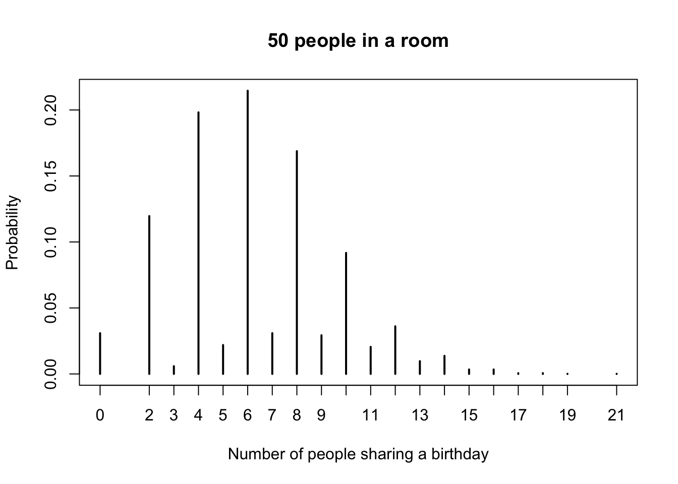
Looking at the pmf, our best estimate is that the most likely outcome is that 6 people in the room share a birthday with someone else, followed closely by 4 and then 8. Note that it is impossible for exactly one person to share a birthday with someone else in the room! It would be preferable for several reasons to have the observation \(P(X = 1) = 0\) listed in the table above, but we leave that for another day.
You toss a coin 100 times. After each toss, either there have been more heads, more tails, or the same number of heads and tails. Let \(X\) be the number of times in the 100 tosses that there were more heads than tails. Estimate the pmf of \(X\).
Before looking at the solution, guess whether the pmf of \(X\) will be centered around 50, or not.
We start by doing a single run of the experiment. Recall that the function cumsum accepts a numeric vector and returns the cumulative sum of the vector. So, cumsum(c(1, 3, -1)) would return c(1, 4, 3).
coin_flips <- sample(c("H", "T"), 100, replace = TRUE) # flip 100 coins
num_heads <- cumsum(coin_flips == "H") # cumulative number of heads so far
num_tails <- cumsum(coin_flips == "T") # cumulative number of tails so far
sum(num_heads > num_tails) # number of times there were more heads than tails
## [1] 0Now, we put that inside of replicate.
simdata <- replicate(100000, {
  coin_flips <- sample(c("H", "T"), 100, replace = TRUE)
  num_heads <- cumsum(coin_flips == "H")
  num_tails <- cumsum(coin_flips == "T")
  sum(num_heads > num_tails)
})
pmf <- proportions(table(simdata))
When we have this many possible outcomes, it is easier to view a plot of the pmf than to look directly at the table of probabilities.
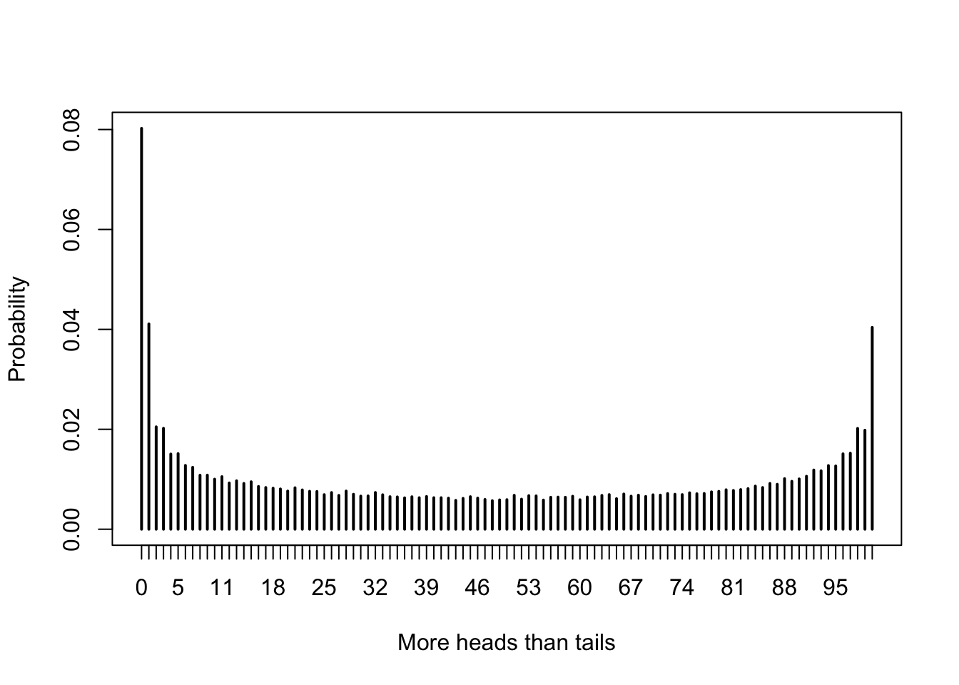
The most likely outcome (by far) is that there are never more heads than tails in the 100 tosses of the coin. This result can be surprising, even to experienced mathematicians.
Suppose you have a bag full of marbles; 50 are red and 50 are blue. You are standing on a number line, and you draw a marble out of the bag. If you get red, you go left one unit. If you get blue, you go right one unit. This is called a random walk. You draw marbles up to 100 times, each time moving left or right one unit. Let \(X\) be the number of marbles drawn from the bag until you return to 0 for the first time. The rv \(X\) is called the first return time since it is the number of steps it takes to return to your starting position.
Estimate the pmf of \(X\).
## [1] -1 1 1 -1 1 -1 1 -1 1 1## [1] -1 0 1 0 1 0 1 0 1 2## [1] 2 4 6 8 22 28 30 32 34 36 86 94 96 98 100## [1] 2Now, we just need to table it like we did before.
simdata <- replicate(10000, {
  movements <- sample(rep(c(1, -1), times = 50), 100, replace = FALSE)
  min(which(cumsum(movements) == 0))
})
pmf <- proportions(table(simdata))
plot(pmf,
  main = "First return time for a 100 step random walk",
  xlab = "Steps to return",
  ylab = "Probability"
)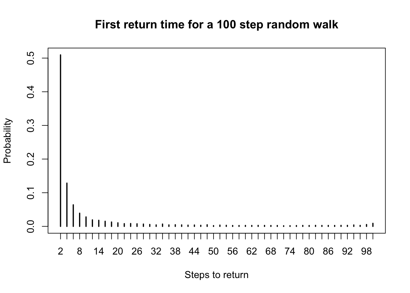
Only even return times are possible (why?). Half the time the first return is after two draws, one of each color. There is a slight bump near 100, when the bag of marbles empties out and the number of red and blue marbles drawn are forced to equalize.
5.3 Estimating continuous distributions
In this section, we show how to estimate the pdf of a continuous rv via simulation. As opposed to the discrete case, we will not get explicit values for the pdf, but we will rather get a graph of it.
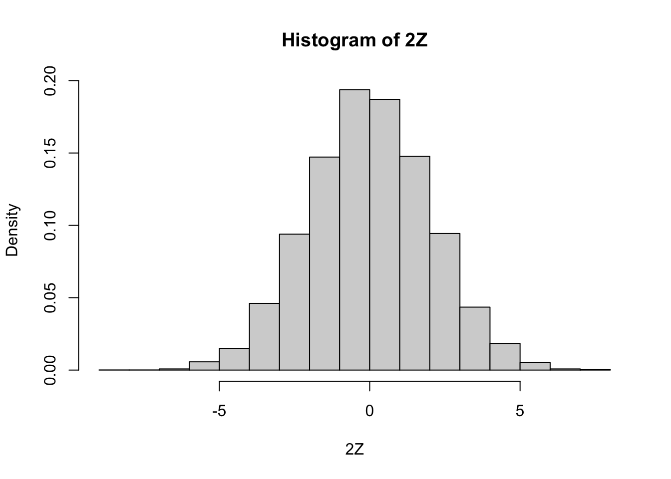
Estimate the pdf of \(2Z\) when \(Z\) is a standard normal random variable
Our strategy is to take a random sample of size 10,000 and use either the density or the hist function to estimate the pdf. As before, we build our sample of size 10,000 up as follows:
A single value sampled from standard normal rv:
We multiply it by 2 to get a single value sampled from \(2Z\).
## [1] 0.03234922Now create 10,000 values of \(2Z\):
We then use density to estimate and plot the pdf of the data:
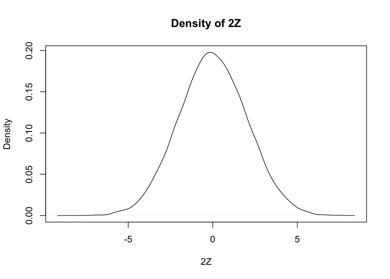
Notice that the most likely outcome of \(2Z\) seems to be 0, just as it is for \(Z\), but that the spread of the distribution of \(2Z\) is twice as wide as the spread of \(Z\).
Alternatively, we could create a histogram of the data, using hist.
We set probability = TRUE to adjust the scale on the y-axis so that the area of each rectangle in the histogram
is the probability that the random variable falls in the interval given by the base of the rectangle.
Given experimental information about a probability density, we wish to compare it to a known theoretical pdf.
A direct way to make this comparison is to plot the estimated pdf on the same graph as the theoretical pdf.
To add a curve to a histogram, density plot, or any plot, use the R function curve.
Compare the pdf of \(2Z\), where \(Z\sim \text{Normal}(0,1)\) to the pdf of a normal random variable with mean 0 and standard deviation 2.
We already saw how to estimate the pdf of \(2Z\), we just need to plot the pdf of \(\text{Normal}(0,2)\) on the same graph27. We show how to do this using both the histogram and the density plot approach. The pdf \(f(x)\) of \(\text{Normal}(0,2)\) is given in R by the function \(f(x) = \text{dnorm}(x,0,2)\).
zData <- 2 * rnorm(10000)
hist(zData,
  probability = TRUE,
  main = "Density and Histogram of 2Z",
  xlab = "2Z"
)
curve(dnorm(x, 0, 2), add = TRUE, col = "red")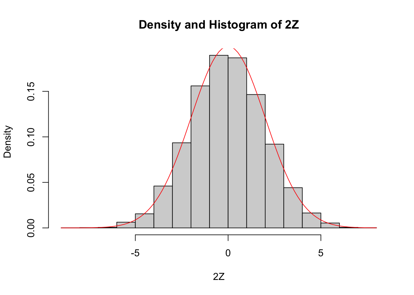
Since the area under of each rectangle in the histogram is approximately the same as the area under the curve over the same interval, this is evidence that \(2Z\) is normal with mean 0 and standard deviation 2. Next, let’s look at the density estimation together with the true pdf of a normal with mean 0 and \(\sigma = 2\).
plot(density(zData),
  xlab = "2Z",
  main = "Density 2Z and Normal(0, 2)"
)
curve(dnorm(x, 0, 2), add = TRUE, col = "red")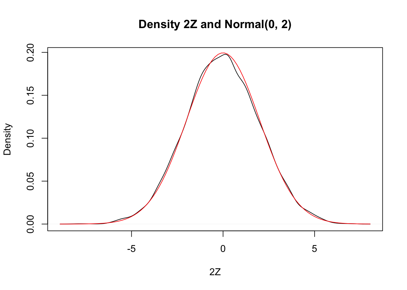
Wow! Those look really close to the same thing! This is again evidence that \(2Z \sim \text{Normal}(0, 2)\).
It would be a good idea to label the two curves in our plots, but that sort of finesse is easier with ggplot, which will be discussed in Chapter 7. Also in Chapter 7, we introduce qq plots, which are a more accurate (but less intuitive) way to compare continuous distributions.
Having observed that the distribution of \(2Z\) matches a normal rv with mean 0 and sd 2, we generalize to a simple theorem. An even more general version of this is stated later, in Theorem 5.4.
Let \(X\) be a normal random variable with mean \(\mu\) and standard deviation \(\sigma\). Then \(aX + b\) is a normal random variable with mean \(a\mu + b\) and standard deviation \(a\sigma\).
Let \(Z\) be a standard normal random variable. By Definition 4.19, \(X = \sigma Z + \mu\), and so \[ aX + b = a(\sigma Z + \mu) + b = (a\sigma)Z + (a\mu + b) \] which is a normal random variable with mean \(a\mu + b\) and standard deviation \(a\sigma\).
Estimate via simulation the pdf of \(\log\bigl(\left|Z\right|\bigr)\) when \(Z\) is standard normal.
expData <- log(abs(rnorm(10000)))
plot(density(expData),
  main = "Density of log|Z|",
  xlab = "log|Z|"
)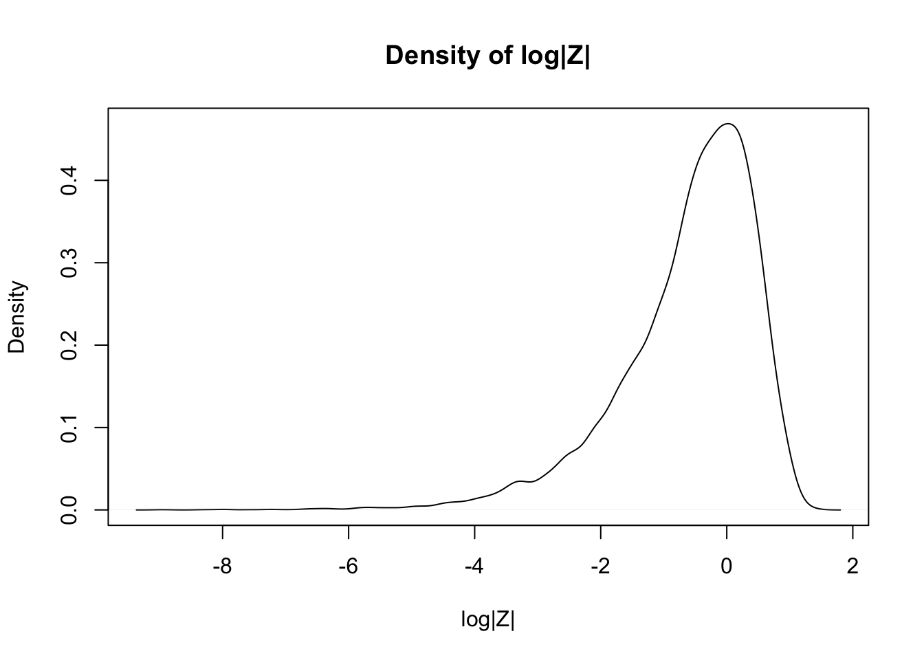
The simulations in Examples 5.10 and 5.12 worked well because the pdfs of \(2Z\) and of \(\log\bigl(\left|Z\right|\bigr)\) are continuous functions. For pdfs with discontinuities, the density estimation tends to misleadingly smooth out the jumps in the function.
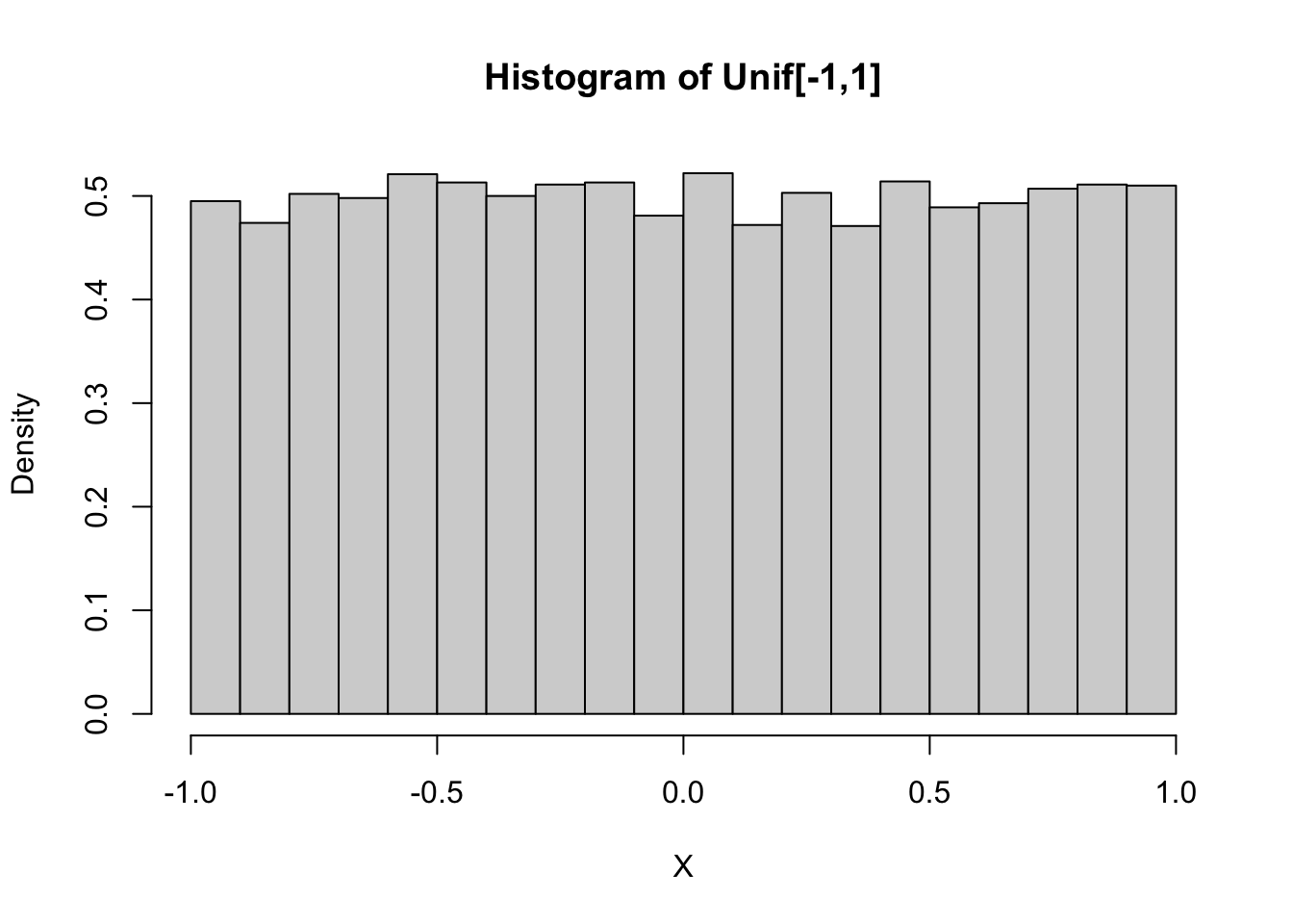
Estimate the pdf of \(X\) when \(X\) is uniform on the interval \([-1,1]\).
unifData <- runif(10000, -1, 1)
plot(density(unifData),
  main = "Density of Unif[-1,1]",
  xlab = "X"
)
curve(dunif(x, -1, 1), add = TRUE, col = "red")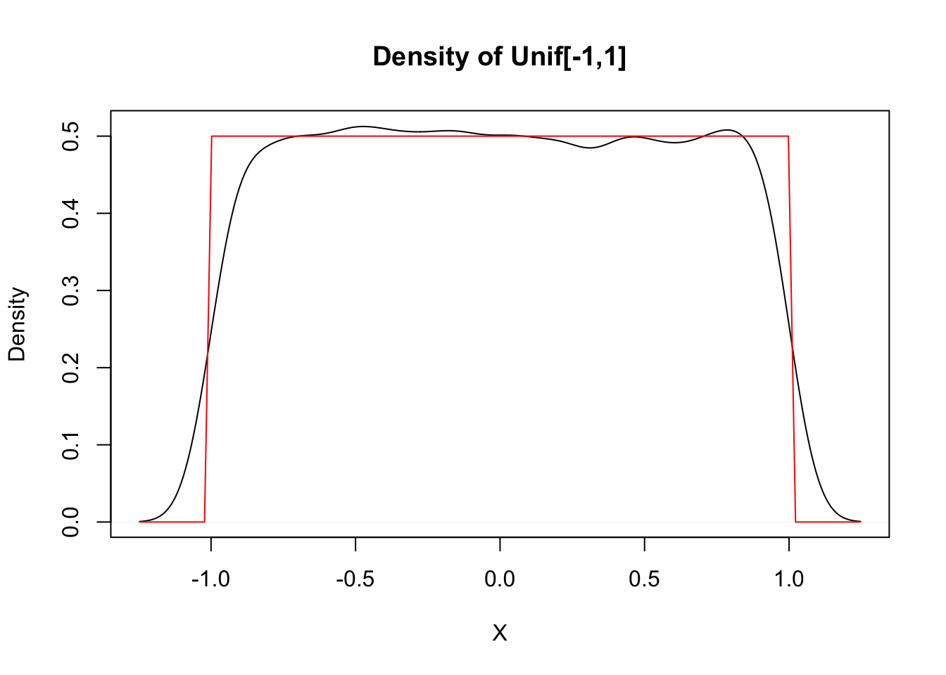
This distribution should be exactly 0.5 between -1 and 1, and zero everywhere else, as shown by the theoretical distribution in red. The simulation is reasonable in the middle, but the discontinuities at the endpoints are not shown well. Increasing the number of data points helps, but does not fix the problem. Compare with the histogram approach, which seems to work better when the data comes from a distribution with a jump discontinuity.
Let’s meet an important distribution, the \(\chi^2\) (chi-squared)
distribution. In fact, \(\chi^2\) is a family of distributions controlled by a parameter called
the degrees of freedom, usually abbreviated df.
The distname for a \(\chi^2\) rv is chisq, and dchisq requires the degrees of freedom to be specified using the df parameter.
Let \(Z\) be a standard normal rv. Find the pdf of \(Z^2\) and compare it to the pdf of the \(\chi^2\) rv with one df on the same plot.
zData <- rnorm(10000)^2
hist(zData,
  probability = T,
  main = "Density and Histogram of Z^2",
  xlab = "Z^2"
)
curve(dchisq(x, df = 1), add = TRUE, col = "red")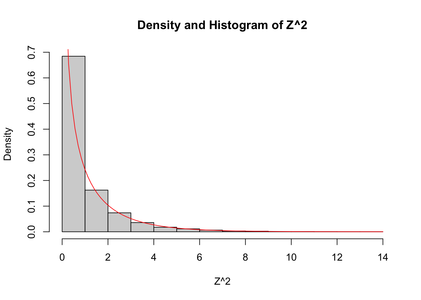
As you can see, the estimated density follows the true histogram quite well. This is evidence that \(Z^2\) is, in fact, chi-squared. Notice that \(\chi^2\) with one df has a vertical asymptote at \(x = 0\).
Let \(Z\) be a normal random variable with mean 0 and standard deviation 1. Then, \(Z^2\) is a chi-squared random variable with 1 degree of freedom.
Estimate the pdf of \(X + Y\) when \(X\) and \(Y\) are independent exponential random variables with rate 2.
simdata <- replicate(10000, {
  x <- rexp(1, 2)
  y <- rexp(1, 2)
  x + y
})
hist(simdata,
  probability = TRUE,
  main = "Histogram of Sum of Exponentials",
  xlab = "X + Y"
)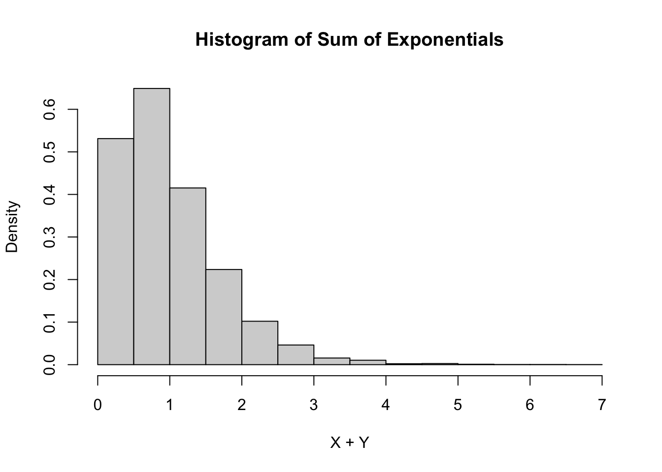
The sum of exponential random variables follows what is called a gamma distribution. The gamma distribution is represented in R via the base gamma together with the typical prefixes dpqr. A gamma random variable has two parameters, the shape and the rate. It turns out, see Exercise 5.21, that
- the sum of independent gamma random variables with the same rate
rateand shapess1ands2is again gamma with raterateand shapes1 + s2, and - a gamma random variable with shape 1 is exponential.
Combining those two facts means that the sum of the independent exponential random variables with rate 2 in this example should be gamma with shape 2 and rate 2.
hist(simdata,
  probability = TRUE,
  main = "Sum of Exponentials is Gamma",
  xlab = "X + Y"
)
curve(dgamma(x, shape = 2, rate = 2), add = T, col = 2)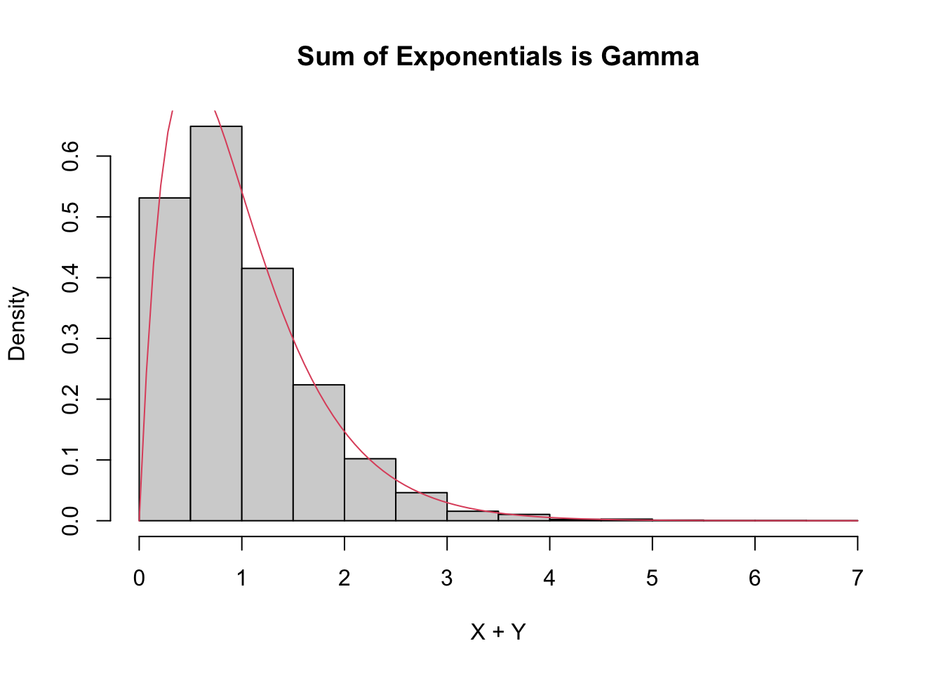
Estimate the density of \(X_1 + X_2 + \cdots + X_{20}\) when all of the \(X_i\) are independent exponential random variables with rate 2.
This one is trickier and is our first example where it is easier to use replicate to create the data. Let’s build up the experiment that we are replicating from the ground up.
Here’s the experiment of summing 20 exponential rvs with rate 2:
## [1] 3.436337Now replicate it (10 times to test):
##  [1] 12.214462 10.755431 13.170513  4.983875 10.259718  7.937500
##  [7] 11.313176 10.192818  7.386954 10.748529
Of course, we don’t want to just replicate it 10 times, we need about 10,000 data points to get a good density estimate.
sumExpData <- replicate(10000, sum(rexp(20, 2)))
plot(density(sumExpData),
  main = "Density of Sum of 20 Exponentials",
  xlab = "X1 + ... + X20"
)
curve(dgamma(x, shape = 20, rate = 2), add = T, col = 2)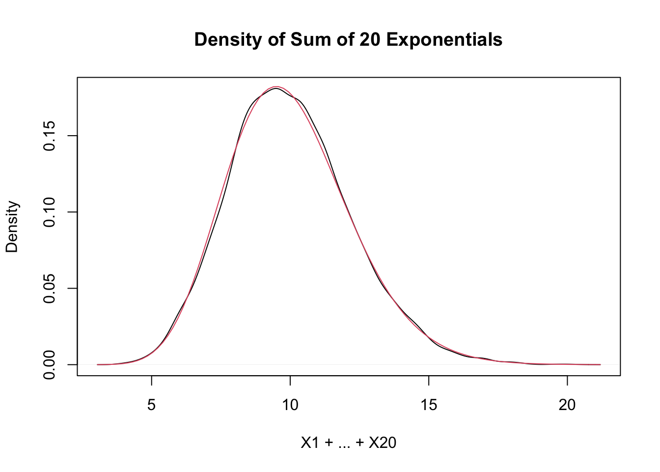
As explained in the previous example, this is exactly a gamma random variable with rate 2 and shape 20, and it is also starting to look like a normal random variable! Exercise 5.26 asks you to fit a normal curve to this distribution.
5.4 The Central Limit Theorem
Random variables \(X_1,\ldots,X_n\) are called independent identically distributed or iid if each pair of variables are independent, and each \(X_i\) has the same probability distribution.
All of the r + distname functions (rnorm, rexp, etc.) produce iid random variables.
In the real world, iid rvs are produced by randomly sampling a population.
As long as the population size is much larger than \(n\),
the sampled values will be independent, and all will have the same probability distribution
as the population distribution. In practice, it is quite hard to sample randomly from a real population.
Let \(X_1, \dotsc, X_n\) be a random sample. A random variable \(Y = h(X_1, \dotsc, X_n)\) that is derived from the random sample is called a sample statistic or sometimes just a statistic. The probability distribution of \(Y\) is called a sampling distribution.
Three of the most important statistics are the sample mean, sample variance, and sample sd.
Assume \(X_1,\ldots,X_n\) are independent and identically distributed with mean \(\mu\) and standard deviation \(\sigma\). Define:
- The sample mean \[ \overline{X} = \frac{X_1 + \dotsb + X_n}{n}. \]
- The sample variance \[ S^2 = \frac 1{n-1} \sum_{i=1}^n (X_i - \overline{X})^2 \]
- The sample standard deviation is \(S\), the square root of the sample variance.
These three statistics are computed in R with the commands mean, var, and sd that we have been using all along.
A primary goal of statistics is to learn something about a population (the distribution of the \(X_i\)’s) by studying sample statistics. We can make precise statements about a population from a random sample because it is possible to describe the sampling distributions of statistics like \(\overline{X}\) and \(S\) even in the absence of information about the distribution of the \(X_i\). The most important example of this phenomenon is the Central Limit Theorem, which is fundamental to statistical reasoning.
In its most straightforward version, the Central Limit Theorem is a statement about the statistic \(\overline{X}\), the sample mean. It says that for large samples, the probability distribution of \(\overline{X}\) becomes normal.
Let \(X_1,\ldots,X_n\) be iid rvs with finite mean \(\mu\) and standard deviation \(\sigma\). Then \[ \frac{\overline{X} - \mu}{\sigma/\sqrt{n}} \to Z \qquad \text{as}\ n \to \infty \] where \(Z\) is a standard normal rv.
We will not prove Theorem 5.3, but we will do simulations for several examples. They will all follow a similar format.
Let \(X_1,\ldots,X_{30}\) be independent Poisson random variables with rate 2. From our knowledge of the Poisson distribution, each \(X_i\) has mean \(\mu = 2\) and standard deviation \(\sigma = \sqrt{2}\). The central limit theorem says that \[ \frac{\overline{X} - 2}{\sqrt{2}/\sqrt{30}} \] will be approximately normal with mean 0 and standard deviation 1 if \(n = 30\) is a large enough sample size. We will investigate later how to determine what a large enough sample size would be, but for now we assume that for this case, \(n = 30\) is big enough. Let us check this with a simulation.
This is a little but more complicated than our previous examples, but the idea is still the same. We create an experiment which computes \(\overline{X}\) and then transforms by subtracting 2 and dividing by \(\sqrt{2}/\sqrt{30}\).
Here is a single experiment:
## [1] 1.032796Now, we replicate and plot:
poisData <- replicate(10000, {
xbar <- mean(rpois(30, 2))
(xbar - 2) / (sqrt(2) / sqrt(30))
})
plot(density(poisData),
main = "Standardized sum of Poisson Compared to Normal",
xlab = "x"
)
curve(dnorm(x), add = T, col = 2)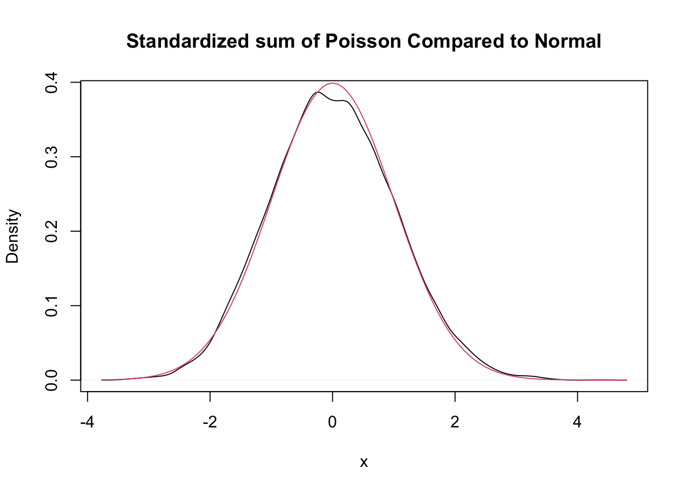
Very close!
Let \(X_1,\ldots,X_{50}\) be independent exponential random variables with rate 1/3. From our knowledge of the exponential distribution, each \(X_i\) has mean \(\mu = 3\) and standard deviation \(\sigma = 3\). The central limit theorem says that \[ \frac{\overline{X} - 3}{3/\sqrt{n}} \] is approximately normal with mean 0 and standard deviation 1 when \(n\) is large. We check this with a simulation in the case \(n = 50\). Again, we can either use histograms or density estimates for this, but this time we choose to use density estimates.
expData <- replicate(10000, {
  dat <- mean(rexp(50, 1 / 3))
  (dat - 3) / (3 / sqrt(50))
})
plot(density(expData),
  main = "Standardized sum of exponentials compared to normal",
  xlab = "x"
)
curve(dnorm(x), add = T, col = 2)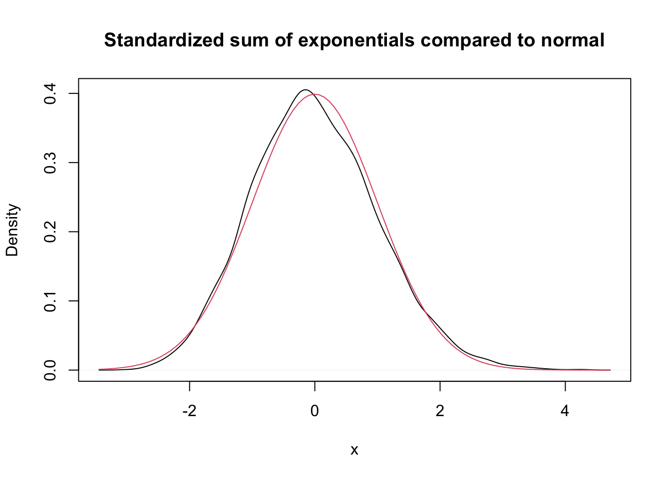
The Central Limit Theorem says that, if you take the mean of a large number of independent samples, then the distribution of that mean will be approximately normal. How large does \(n\) need to be in practice?
- If the population you are sampling from is symmetric with no outliers, a good approximation to normality appears after as few as 15-20 samples.
- If the population is moderately skew, such as exponential or \(\chi^2\), then it can take between 30-50 samples before getting a good approximation.
- Data with extreme skewness, such as some financial data where most entries are 0, a few are small, and even fewer are extremely large, may not be appropriate for the central limit theorem even with 500 samples (see Example 5.22).
There are versions of the Central Limit Theorem available when the \(X_i\) are not iid, but outliers of sufficient size will cause the distribution of \(\overline{X}\) to not be normal, see Exercise 5.31.
A distribution for which sample size of \(n = 500\) is not sufficient for good approximation via normal distributions.
We create a distribution that consists primarily of zeros, but has a few modest sized values and a few large values:
# Start with lots of zeros
skewdata <- replicate(2000, 0)
# Add a few moderately sized values
skewdata <- c(skewdata, rexp(200, 1 / 10))
# Add a few large values
skewdata <- c(skewdata, seq(100000, 500000, 50000))

mu <- mean(skewdata)
sig <- sd(skewdata)
We use sample to take a random sample of size \(n\) from this distribution. We take the mean, subtract the true mean of the distribution, and divide by \(\sigma/\sqrt{n}\). We replicate that 10000 times to estimate the sampling distribution. Here are the plots when \(\overline{X}\) is the
mean of a sample of size 100:
n <- 100

skewSample <- replicate(10000, {
  dat <- mean(sample(skewdata, n, TRUE))
  (dat - mu) / (sig / sqrt(n))
})
hist(skewSample,
  probability = T,
  main = "Histogram of Standardized Mean of 100 Samples",
  xlab = "X"
)
curve(dnorm(x), add = T, col = 2)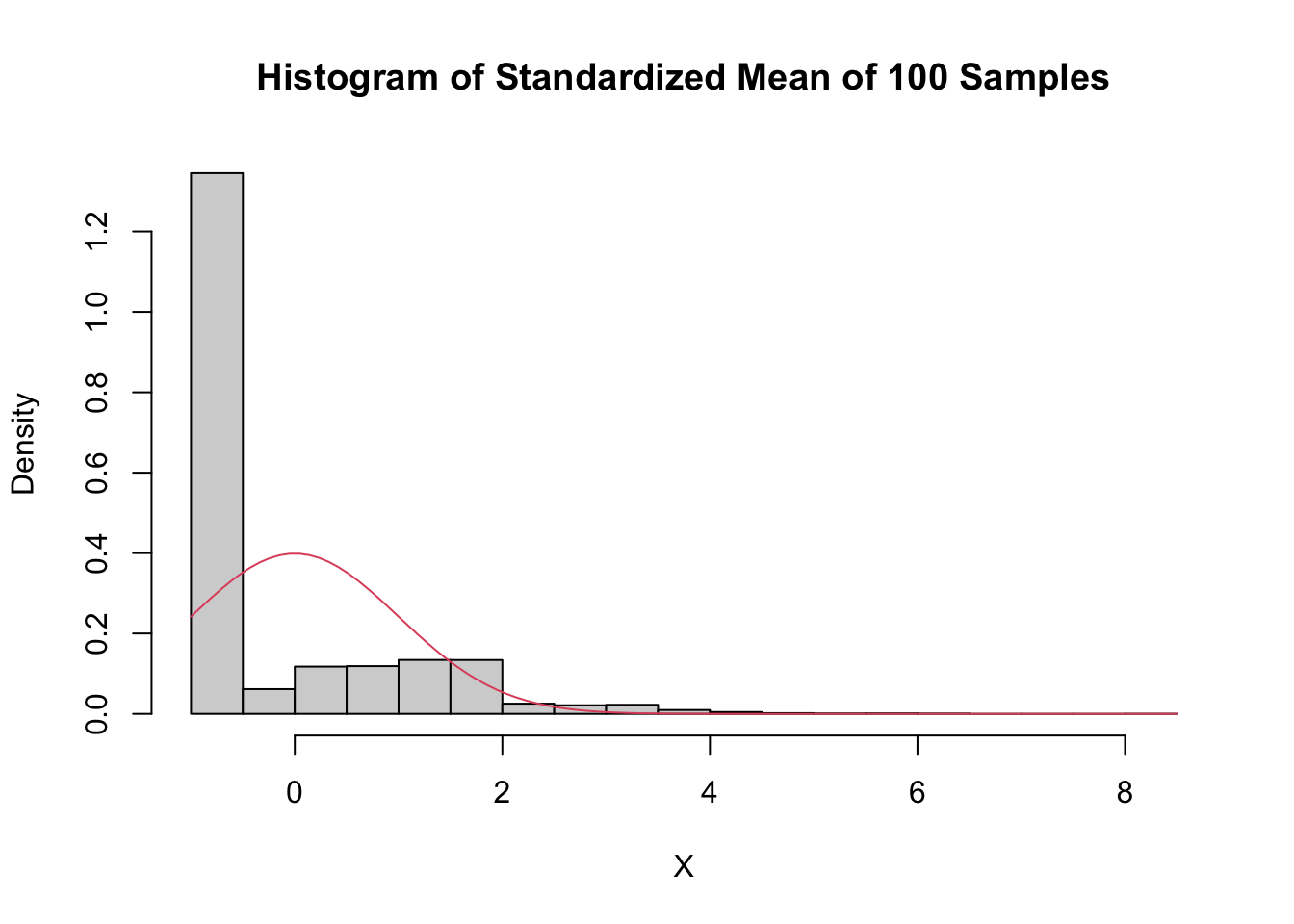
When \(\overline{X}\) is the mean of a sample of size 500:
n <- 500

skewSample <- replicate(10000, {
  dat <- mean(sample(skewdata, n, TRUE))
  (dat - mu) / (sig / sqrt(n))
})

hist(skewSample,
  probability = T,
  main = "Histogram of Standardized Mean of 500 Samples",
  xlab = "x"
)
curve(dnorm(x), add = T, col = 2)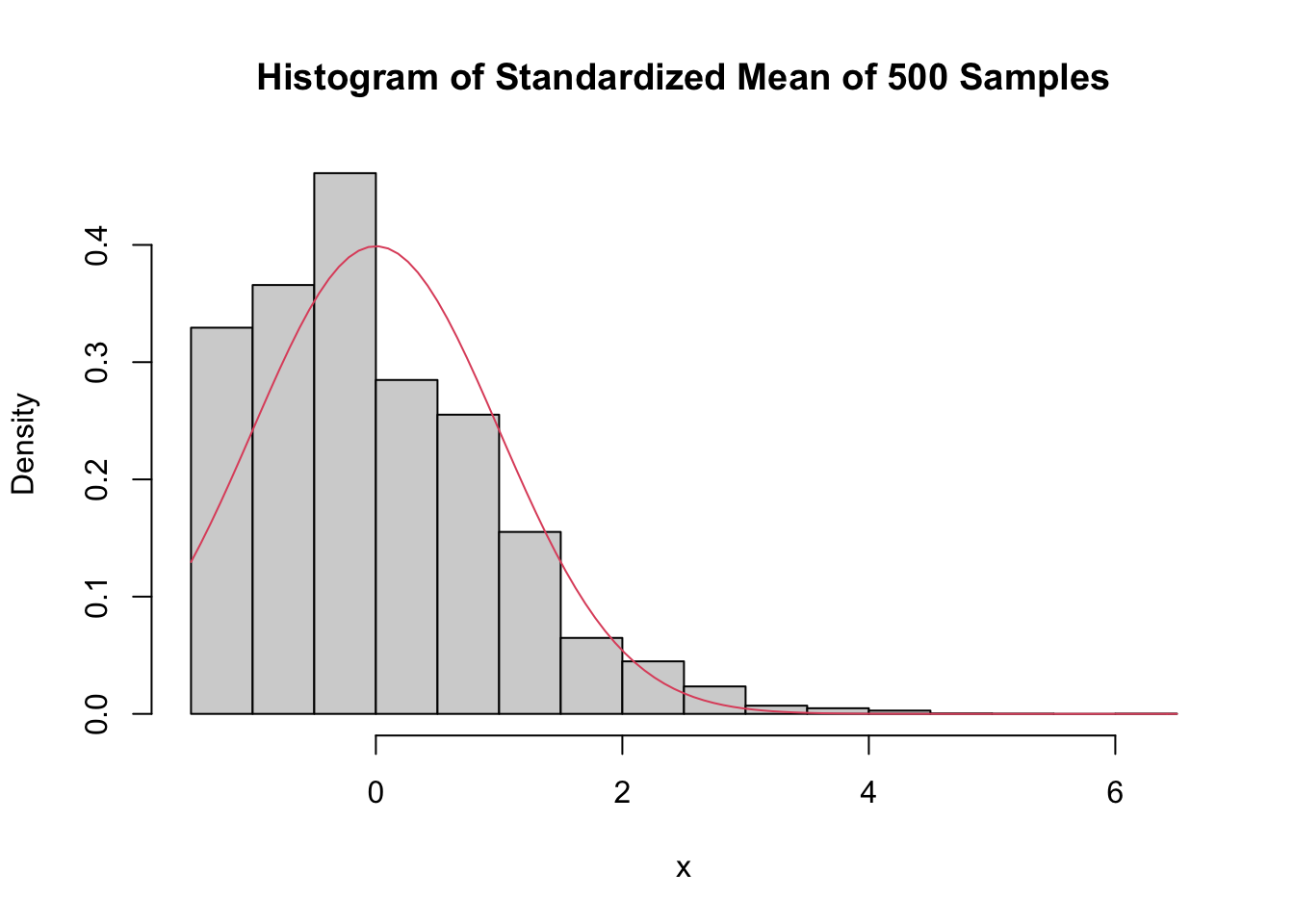
Even with a sample size of 500, the density is still far from the normal distribution, especially the lack of left tail. Of course, the Central Limit Theorem is still true, so \(\overline{X}\) must become normal if we choose \(n\) large enough. Here is the distribution when \(n = 5000\):
n <- 5000

skewSample <- replicate(10000, {
  dat <- mean(sample(skewdata, n, TRUE))
  (dat - mu) / (sig / sqrt(n))
})

hist(skewSample,
  probability = T,
  main = "Histogram of Standardized Mean of 5000 Samples",
  xlab = "x"
)
curve(dnorm(x), add = T, col = 2)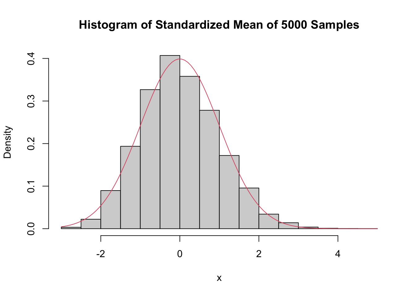
There may still be a slight skewness in this picture, but it is finally close to normal.
5.5 Sampling distributions
We describe the distributions \(t\), \(\chi^2\) and \(F\) in the context of samples from normal rv. The emphasis is on understanding the relationships between the rvs and how they come about from \(\overline{X}\) and \(S\). Your goal should be to get comfortable with the idea that sample statistics have known distributions. You may not be able to prove it, but hopefully won’t be surprised either. We will use density estimation extensively to illustrate the relationships.
5.5.1 Linear combination of normal rv’s
Let \(X_1,\ldots,X_n\) be rvs with means \(\mu_1,\ldots,\mu_n\) and variances \(\sigma_i^2\). Form the linear combination \(a_1 X_1 + \dotsb + a_n X_n\) of these variables with coefficients \(a_1, \dotsc a_n\). Then by Theorem 3.8 \[ E[\sum a_i X_i] = \sum a_i E[X_i] \] and if \(X_1, \ldots, X_n\) are independent, then by Theorem 3.10 \[ \text{Var}(\sum a_i X_i) = \sum a_i^2 \text{Var}(X_i) \]
An important special case is when \(X_1,\ldots,X_n\) are iid with mean \(\mu\) and variance \(\sigma^2\), then \(\overline{X}\) has mean \(\mu\) and variance \(\sigma^2/n\).
These statements describe the mean and variance of the linear combination. The Central Limit Theorem then tells you something about its probability distribution. However, when the \(X_i\) are indepentent and normal, much more can be said. The key fact (which we will not prove) is that the sum of independent normal rvs is normal.
Let \(X_1,\ldots,X_n\) be independent normal rvs with means \(\mu_1,\ldots,\mu_n\) and variances \(\sigma_1^2,\ldots,\sigma_n^2\). Then, \[ \sum_{i=1}^n a_i X_i \] is normal with mean \(\sum a_i \mu_i\) and variance \(\sum a_i^2 \sigma_i^2\).
You will be asked to verify this via estimating densities in special cases in the exercises. The special case that is very interesting is the following:
Let \(X_1,\ldots,X_n\) be independent identically distributed normal rvs with common mean \(\mu\) and variance \(\sigma^2\). Then \[ \frac{\overline{X} - \mu}{\sigma/\sqrt{n}} = Z \] is standard normal(0,1).
Theorem 5.5 is similar to the Central Limit Theorem in form, except that when we start with normal rv \(X_1, \dotsc, X_n\) there is no need for a limit. The result is true exactly, for any value of \(n\).
5.5.2 Chi-squared
Let \(Z\) be a standard normal random variable. An rv with the same distribution as \(Z^2\) is called a Chi-squared random variable with one degree of freedom.
Let \(Z_1, \dotsc, Z_n\) be \(n\) iid standard normal random variables. Then an rv with the same distribution as \(Z_1^2 + \dotsb + Z_n^2\) is called a Chi-squared random variable with \(n\) degrees of freedom.
The sum of \(n\) independent \(\chi^2\) rv’s with 1 degree of freedom is a \(\chi^2\) rv with \(n\) degrees of freedom. More generally, the sum of a \(\chi^2\) with \(\nu_1\) degrees of freedom and a \(\chi^2\) with \(\nu_2\) degrees of freedom is \(\chi^2\) with \(\nu_1 + \nu_2\) degrees of freedom.
Let’s check by estimating pdfs that the sum of a \(\chi^2\) with 2 df and a \(\chi^2\) with 3 df is a \(\chi^2\) with 5 df.
chi2Data <- replicate(10000, rchisq(1, 2) + rchisq(1, 3))
hist(chi2Data,
  probability = TRUE,
  main = "Histogram of sum of Chi^2 Random Variables",
  xlab = "x + y"
)
curve(dchisq(x, df = 5), add = T, col = 2)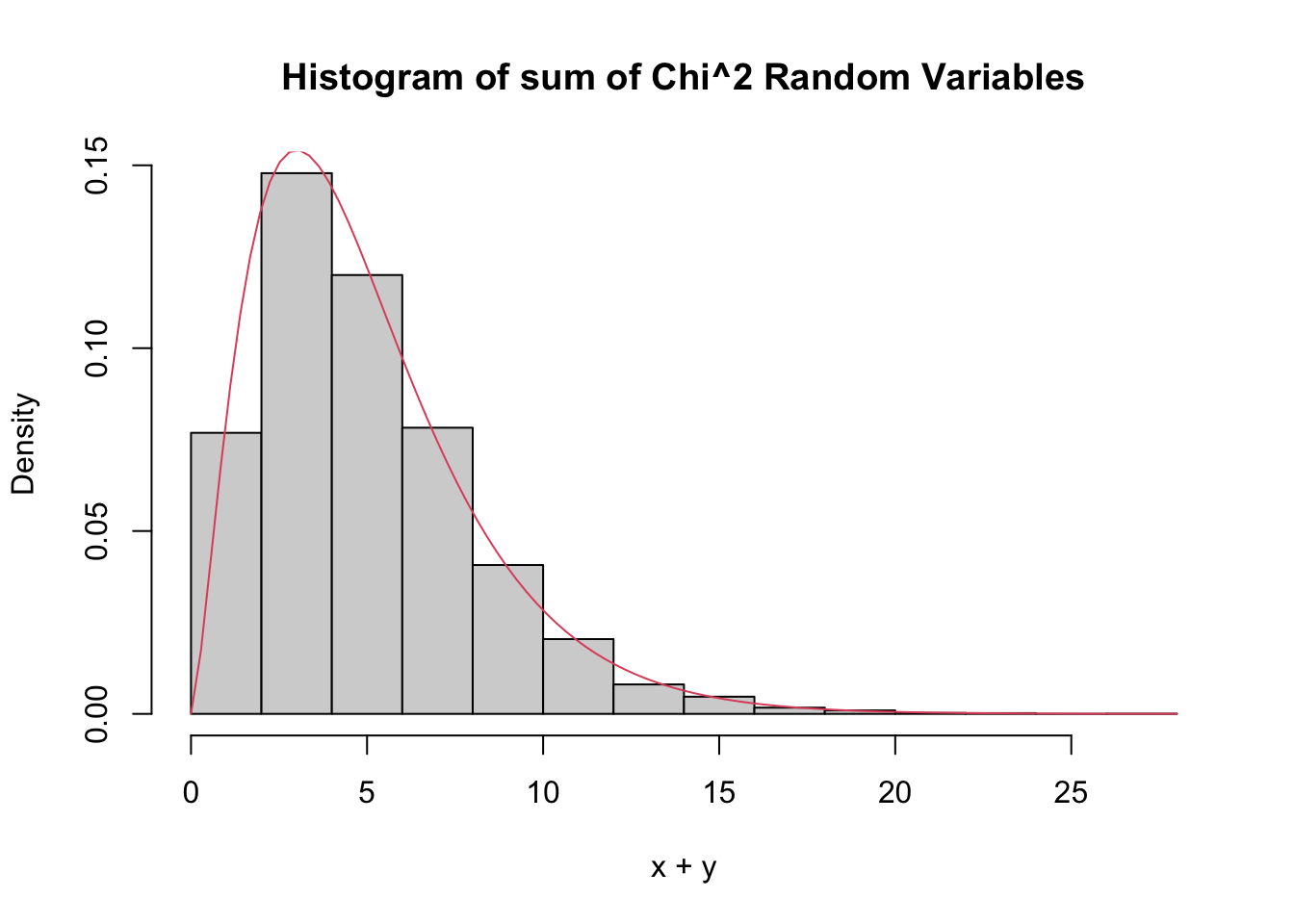
The \(\chi^2\) distribution is important for understanding the sample standard deviation.
If \(X_1,\ldots,X_n\) are iid normal rvs with mean \(\mu\) and standard deviation \(\sigma\), then \[ \frac{n-1}{\sigma^2} S^2 \] has a \(\chi^2\) distribution with \(n-1\) degrees of freedom.
We provide a heuristic and a simulation as evidence that Theorem 5.6 is true. Additionally, in Exercise 5.36 you are asked to prove Theorem 5.6 in the case that \(n = 2\).
Heuristic argument: Note that \[ \frac{n-1}{\sigma^2} S^2 = \frac 1{\sigma^2}\sum_{i=1}^n (X_i - \overline{X})^2 \\ = \sum_{i=1}^n \bigl(\frac{X_i - \overline{X}}{\sigma}\bigr)^2 \] Now, if we had \(\mu\) in place of \(\overline{X}\) in the above equation, we would have exactly a \(\chi^2\) with \(n\) degrees of freedom. Replacing \(\mu\) by its estimate \(\overline{X}\) reduces the degrees of freedom by one, but it remains \(\chi^2\).
For the simulation, we estimate the density of \(\frac{n-1}{\sigma^2} S^2\) and compare it to that of a \(\chi^2\) with \(n-1\) degrees of freedom, in the case that \(n = 4\), \(\mu = 3\) and \(\sigma = 9\).
sdData <- replicate(10000, 3 / 81 * sd(rnorm(4, 3, 9))^2)
hist(sdData,
  probability = TRUE,
  main = "Histogram of Sample Variance Compared to Chi^2",
  xlab = "S",
  ylim = c(0, .25)
)
curve(dchisq(x, df = 3), add = T, col = 2)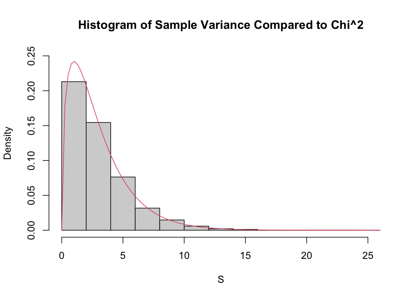
5.5.3 The \(t\) distribution
This section introduces Student’s \(t\) distribution. The distribution is named after William Gosset, who published under the pseudonym “Student” while working at the Guinness Brewery in the early 1900’s.
If \(Z\) is a standard normal(0,1) rv, \(\chi^2_\nu\) is a Chi-squared rv with \(\nu\) degrees of freedom, and \(Z\) and \(\chi^2_\nu\) are independent, then
\[ t_\nu = \frac{Z}{\sqrt{\chi^2_\nu/\nu}} \]
is distributed as a \(t\) random variable with \(\nu\) degrees of freedom .
If \(X_1,\ldots,X_n\) are iid normal rvs with mean \(\mu\) and sd \(\sigma\), then \[ \frac{\overline{X} - \mu}{S/\sqrt{n}} \] is \(t\) with \(n-1\) degrees of freedom.
Note that \(\frac{\overline{X} - \mu}{\sigma/\sqrt{n}}\) is normal(0,1). So, replacing \(\sigma\) with \(S\) changes the distribution from normal to \(t\).
\[ \frac{Z}{\sqrt{\chi^2_{n-1}/n}} = \frac{\overline{X} - \mu}{\sigma/\sqrt{n}}*\sqrt{\frac{\sigma^2 (n-1)}{S^2(n-1)}}\\ = \frac{\overline{X} - \mu}{S/\sqrt{n}} \] Where we have used that \((n - 1) S^2/\sigma^2\) is \(\chi^2\) with \(n - 1\) degrees of freedom.
Estimate the pdf of \(\frac{\overline{X} - \mu}{S/\sqrt{n}}\) in the case that \(X_1,\ldots,X_6\) are iid normal with mean 3 and standard deviation 4, and compare it to the pdf of the appropriate \(t\) random variable.
tData <- replicate(10000, {
  normData <- rnorm(6, 3, 4)
  (mean(normData) - 3) / (sd(normData) / sqrt(6))
})
hist(tData,
  probability = TRUE,
  ylim = c(0, .37),
  main = "Histogram of t",
  xlab = "t"
)
curve(dt(x, df = 5), add = TRUE, col = 2)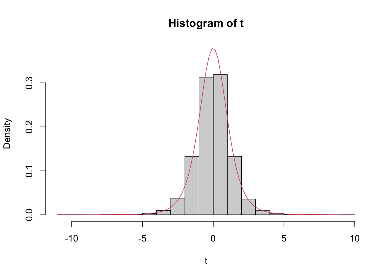
We see a very good agreement.
5.5.4 The F distribution
An \(F\) distribution has the same density function as \[ F_{\nu_1, \nu_2} = \frac{\chi^2_{\nu_1}/\nu_1}{\chi^2_{\nu_2}/\nu_2} \] We say \(F\) has \(\nu_1\) numerator degrees of freedom and \(\nu_2\) denominator degrees of freedom.
One example of this type is: \[ \frac{S_1^2/\sigma_1^2}{S_2^2/\sigma_2^2} \] where \(X_1,\ldots,X_{n_1}\) are iid normal with standard deviation \(\sigma_1\) and \(Y_1,\ldots,Y_{n_2}\) are iid normal with standard deviation \(\sigma_2.\)
5.5.5 Summary
- \(aX+ b\) is normal with mean \(a\mu + b\) and standard deviation \(a\sigma\) if \(X\) is normal with mean \(\mu\) and sd \(\sigma\).
- \(\frac{X - \mu}{\sigma}\sim Z\) if \(X\) is Normal(\(\mu, \sigma\)).
- \(\frac{\overline{X} - \mu}{\sigma/\sqrt{n}} \sim Z\) if \(X_1,\ldots,X_n\) iid normal(\(\mu, \sigma\))
- \(\lim_{n\to \infty} \frac{\overline{X} - \mu}{\sigma/\sqrt{n}} \sim Z\) if \(X_1,\ldots,X_n\) iid with finite variance.
- \(Z^2 \sim \chi^2_1\)
- \(\chi^2_\nu + \chi^2_\eta \sim \chi^2_{\nu + \eta}\) if independent
- \(\frac{(n-1)S^2}{\sigma^2} \sim \chi^2_{n-1}\) when \(X_1,\ldots,X_n\) iid normal.
- \(\frac Z{\sqrt{\chi^2_\nu/\nu}} \sim t_\nu\) if independent
- \(\frac{\overline{X} - \mu}{S/\sqrt{n}}\sim t_{n-1}\) when \(X_1,\ldots,X_n\) iid normal.
- \(\frac{\chi^2_\nu/\nu}{\chi^2_\mu/\mu} \sim F_{\nu, \mu}\) if independent
- \(\frac{S_1^2/\sigma_1^2}{S_2^2/\sigma_2^2} \sim F_{n_1 - 1, n_2 - 1}\) if \(X_1,\ldots,X_{n_1}\) iid normal with sd \(\sigma_1\) and \(Y_1,\ldots,Y_{n_2}\) iid normal with sd \(\sigma_2\).
5.6 Point estimators
This section explores the definition of sample mean and (especially) sample variance, in the more general context of point estimators and their properties.
Suppose that a random variable \(X\) depends on some parameter \(\beta\). In many instances we do not know \(\beta,\) but are interested in estimating it from observations of \(X\).
If \(X_1, \ldots, X_n\) are iid with the same distribution as \(X\), then a point estimator for \(\beta\) is a function \(\hat\beta = h(X_1, \ldots, X_n)\).
Normally the value of \(\hat \beta\) represents our best estimate of the parameter \(\beta\), based on the data. Note that \(\hat \beta\) is a random variable, and since \(\hat \beta\) is derived from \(X_1, \dotsc, X_n\), \(\hat\beta\) is a sample statistic and has a sampling distribution.
The two point estimators that we are interested in in this section are the sample mean and sample variance. The sample mean \(\overline{X}\) is a point estimate for the mean of a random variable, and the sample variance \(S^2\) is a point estimator for the variance of an rv.
Recall that the definition of the mean of a discrete rv with possible values \(x_i\) is \[ E[X] = \mu = \sum_{i=1}^n x_i p(x_i) \] If we are given data \(x_1,\ldots,x_n\), it is natural to assign \(p(x_i) = 1/n\) for each of those data points to create a new random variable \(X_0\), and we obtain \[ E[X_0] = \frac 1n \sum_{i=1}^n x_i = \overline{x} \] This is a natural choice for our point estimator for the mean of the rv \(X\), as well. \[ \hat \mu = \overline{x} = \frac 1n \sum_{i=1}^n x_i \]
Continuing in the same way, if we are given data \(x_1,\ldots,x_n\) and we wish to estimate the variance, then we could create a new random variable \(X_0\) whose possible outcomes are \(x_1,\ldots,x_n\) with probabilities \(1/n\) and compute
\[ \sigma^2 = E[(X- \mu)^2] = \frac 1n \sum_{i=1}^n (x_i - \mu)^2 \]
This works just fine as long as \(\mu\) is known. However, most of the time, we do not know \(\mu\) and we must replace the true value of \(\mu\) with our estimate from the data. There is a heuristic “degrees of freedom” that each time you replace a parameter with an estimate of that parameter, you divide by one less. Following that heuristic, we obtain \[ \hat \sigma^2 = S^2 = \frac 1{n-1} \sum_{i=1}^n (x_i - \overline{x})^2 \]
5.6.1 Properties of point estimators
The point estimators for \(\mu\) and \(\sigma^2\) are random variables themselves, since they are computed using a random sample from a distribution. As such, they also have distributions, means and variances. One desirable property of point estimators is that they be unbiased.
A point estimator \(\hat \beta\) for \(\beta\) is an unbiased estimator if \(E[\hat \beta] = \beta\).
Intuitively, “unbiased” means that the estimator does not consistently underestimate or overestimate the parameter it is estimating. If we were to estimate the parameter over and over again, the average value of the estimates would converge to the correct value of the parameter.
Let \(X_1,\ldots, X_{5}\) be a random sample from a normal distribution with mean 1 and variance 1. Compute \(\overline{x}\) based on the random sample.
## [1] 0.9330305You can see the estimate is pretty close to the correct value of 1, but not exactly 1. However, if we repeat this experiment 10,000 times and take the average value of \(\overline{x}\), that should be very close to 1.
## [1] 1.006326It can be useful to repeat this a few times to see whether it seems to be consistently overestimating or underestimating the mean. In this case, it is not.
For a population with mean \(\mu\), the sample mean \(\overline{X}\) is an unbiased estimator of \(\mu\).
Let \(X_1, \ldots, X_n\) be a sample from the population, so \(E[X_i] = \mu\). Then \[ E[\overline{X}] = E\left[\frac{X_1 + \dotsb + X_n}{n}\right] = \frac{1}{n}\left(E[X_1] + \dotsb + E[X_n]\right) = \mu.\]
Now consider the sample variance \(S^2\). The formula \[ S^2 = \frac {1}{n-1} \sum_{i=1}^n (X_i - \overline{X})^2 \] contains a somewhat surprising division by \(n-1\), since the sum has \(n\) terms. We explore this with simulation.
Let \(X_1,\ldots,X_5\) be a random sample from a normal rv with mean 1 and variance 4. Estimate the variance using \(S^2\).
## [1] 3.393033We see that our estimate is not ridiculous, but not the best either. Let’s repeat this 10,000 times and take the average. (We are estimating \(E[S^2]\).)
## [1] 3.986978Again, repeating this a few times, it seems that we are neither overestimating nor underestimating the value of the variance.
In this example, we see that dividing by \(n\) would lead to a biased estimator.
That is, \(\frac 1n \sum_{i=1}^n (X_i - \overline{X})^2\) is not an unbiased estimator of \(\sigma^2\).
We use replicate twice. On the inside, it is running 10000 simulations. On the outside, it is repeating the overall simulation 7 times.
replicate(
  7,
  mean(replicate(10000, {
    data <- rnorm(5, 1, 2)
    1 / 5 * sum((data - mean(data))^2)
  }))
)
## [1] 3.242466 3.212477 3.231688 3.187677 3.157526 3.218117 3.227146In each of the 7 trials, \(\frac 1n \sum_{i=1}^n (X_i - \overline{X})^2\) underestimates the correct value \(\sigma^2 = 4\) by quite a bit.
In summary, \(S^2\) is an unbiased estimator of the population variance \(\sigma^2\).
5.6.2 Variance of unbiased estimators
From the above, we can see that \(\overline{x}\) and \(S^2\) are unbiased estimators for \(\mu\) and \(\sigma^2\), respectively. There are other unbiased estimator for the mean and variance, however.
The median of a collection of numbers is the middle number, after sorting (or the average of the two middle numbers). When a population is symmetric about its mean \(\mu\), the median is an unbiased estimator of \(\mu\). If the population is not symmetric, the median is not typically an unbiased estimator for \(\mu\), see Exercise 5.37 and Exercise 5.38.
If \(X_1,\ldots,X_n\) is a random sample from a normal rv, then the median of the \(X_i\) is an unbiased estimator for the mean. Moreover, the median seems like a perfectly reasonable thing to use to estimate \(\mu\), and in many cases is actually preferred to the mean.
There is one way, however, in which the sample mean \(\overline{x}\) is definitely better than the median, and that is that the mean has a lower variance than the median. This means that \(\overline{x}\) does not deviate from the true mean as much as the median will deviate from the true mean, as measured by variance.
Let’s do a simulation to illustrate. Suppose you have a random sample of size 11 from a normal rv with mean 0 and standard deviation 1. We estimate the variance of the mean \(\overline{x}\).
## [1] 0.08961579Now we repeat for the median.
## [1] 0.1400155We see that the variance of the mean is lower than the variance of the median. This is a good reason to use the sample mean to estimate the mean of a normal rv rather than using the median, absent other considerations such as outliers.
Vignette: Loops in R
Most tasks in R can be done using the implicit loops described in this section. There are also powerful tools in the purrr package. However, sometimes it is easiest just to write a conventional loop. This vignette explains how to use while loops in the context of simulations.
A while loop repeats one or more statements until a certain condition is no longer met.
It is crucial when writing a while loop that you ensure that the condition to exit the loop will eventually be satisfied! The format looks like this.
## [1] 0
## [1] 1
R sets i to 0 and then checks whether i < 2 (it is). It then prints i and adds one to i.
It checks again - is i < 2? Yes, so it prints i and adds one to it.
At this point i is not less than 2, so R exits the loop.
As an real example of while loops in action, suppose we want to estimate the expected value of a geometric random variable \(X\).
Example 3.13 simulated tossing a fair coin until heads occurs, and counting the number of tails. In that case, \(X\) is geometric with \(p=0.5\) and so has \(E[X] = 1\). The approach was to simulate 100 coin flips and assume that heads would appear before we ran out of flips. The probability of flipping 100 tails in a row is negligible, so 100 flips was enough.
To simulate a geometric rv where \(p\) is small and unknown it may take a large number of trials before observing the first success.
If each Bernoulli trial is actually a complicated calculation, we want to stop as soon as the first success occurs.
Under these circumstances, it is better to use a while loop.
Here is a simulation of flipping a coin until heads, using a while loop.
In each iteration of the loop, we flip the coin with sample, print the result, and then add one to the count num_tails.
num_tails <- 0
coin_toss <- ""
while (coin_toss != "Head") {
  coin_toss <- sample(c("Head", "Tail"), 1)
  print(coin_toss)
  if (coin_toss == "Tail") {
    num_tails <- num_tails + 1
  }
}
## [1] "Tail"
## [1] "Tail"
## [1] "Head"## [1] 2This gives one simulated value of \(X\). In this case we found \(X = 2\), because two tails appeared before the first head. To estimate \(E[X]\),
replicate the experiment.
sim_data <- replicate(10000, {
  num_tails <- 0
  coin_toss <- ""
  while (coin_toss != "Head") {
    coin_toss <- sample(c("Head", "Tail"), 1)
    if (coin_toss == "Tail") {
      num_tails <- num_tails + 1
    }
  }
  num_tails
})
mean(sim_data)
## [1] 0.9847The mean of our simulated data is 0.9847, which agrees with the theoretical value \(E[X] = 1\).
Exercises
Exercises 5.1 - 5.2 require material through Section 5.1.
Let \(Z\) be a standard normal random variable. Estimate via simulation \(P(Z^2 < 2)\).
Let \(X\) and \(Y\) be independent exponential random variables with rate 3. Let \(Z = \max(X, Y)\) be the maximum of \(X\) and \(Y\). a. Estimate via simulation \(P(Z < 1/2)\). b. Estimate the mean and standard deviation of \(Z\).
Exercises 5.3 - 5.12 require material through Section 5.2.
Five coins are tossed and the number of heads \(X\) is counted. Estimate via simulation the pmf of \(X\).
Three dice are tossed and their sum \(X\) is observed. Use simulation to estimate and plot the pmf of \(X\).
Five six-sided dice are tossed and their product is observed. Use the estimated pmf to find the most likely outcome.
Fifty people put their names in a hat. They then all randomly choose one name from the hat. Let \(X\) be the number of people who get their own name. Estimate and plot the pmf of \(X\).
Consider an experiment where 20 balls are placed randomly into 10 urns. Let \(X\) denote the number of urns that are empty.
- Estimate via simulation the pmf of \(X\).
- What is the most likely outcome?
- What is the least likely outcome that has positive probability?
Suppose 6 people, numbered 1-6, are sitting at a round dinner table with a big plate of spaghetti, and a bag containing 5005 red marbles and 5000 blue marbles. Person 1 takes the spaghetti, serves themselves, and chooses a marble. If the marble is red, they pass the spaghetti to the left. If it is blue, they pass the spaghetti to the right. The guests continue doing this until the last person receives the plate of spaghetti. Let \(X\) denote the number of the person holding the spaghetti at the end of the experiment. Estimate the pmf of \(X\).
Suppose you roll a die until the first time you obtain an even number. Let \(X_1\) be the total number of times you roll a 1, and let \(X_2\) be the total number of times that you roll a 2.
- Is \(E[X_1] = E[X_2]\)? (Hint: Use simulation. It is extremely unlikely that you will roll 30 times before getting the first even number, so you can safely assume that the first even occurs inside of 30 rolls.)
- Is the pmf of \(X_1\) the same as the pmf of \(X_2\)?
- Estimate the variances of \(X_1\) and \(X_2\).
Simulate creating independent uniform random numbers in [0,1] and summing them until your cumulative sum is larger than 1. Let \(N\) be the random variable which is how many numbers you needed to sample. For example, if your numbers were 0.35, 0.58, 0.22 you would have \(N = 3\) since the sum exceeds 1 after the third number. What is the expected value of \(N\)?
Recall the Example 5.8 in the text, where we show that the most likely number of times you have more Heads than Tails when a coin is tossed 100 times is zero. Suppose you toss a coin 100 times.
- Let \(X\) be the number of times in the 100 tosses that you have exactly the same number of Heads as Tails. Estimate the expected value of \(X\).
- Let \(Y\) be the number of tosses for which you have more Heads than Tails. Estimate the expected value of \(Y\).
Suppose there are two candidates in an election. Candidate A receives 52 votes and Candidate B receives 48 votes. You count the votes one at a time, keeping a running tally of who is ahead. At each point, either A is ahead, B is ahead or they are tied. Let \(X\) be the number of times that Candidate B is ahead in the 100 tallies.
- Estimate the pmf of \(X\).
- Estimate \(P(X > 50)\).
Exercises 5.13 - 5.24 require material through Section 5.3.
Let \(X\) and \(Y\) be independent uniform random variables on the interval \([0,1]\). Estimate the pdf of \(X+Y\) and plot it.
Let \(X\) and \(Y\) be independent uniform random variables on the interval \([0,1]\). Let \(Z\) be the maximum of \(X\) and \(Y\).
- Plot the pdf of \(Z\).
- From your answer to (a), decide whether \(P(0 \le Z \le 1/3)\) or \(P(1/3\le Z \le 2/3)\) is larger.
Estimate the value of \(a\) such that \(P(a \le Y \le a + 1)\) is maximized when \(Y\) is the maximum value of two independent exponential random variables with mean 2.
Is the product of two normal rvs normal? Estimate via simulation the pdf of the product of \(X\) and \(Y\), when \(X\) and \(Y\) are independent normal random variables with mean 0 and standard deviation 1. How can you determine whether \(XY\) is normal? Hint: you will need to estimate the mean and standard deviation.
The minimum of two independent exponential rv’s with mean 2 is an exponential rv. Use simulation to determine what the rate is.
The sum of two independent chi-squared rv’s with 2 degrees of freedom is either exponential or chi-squared. Which one is it? What is the parameter associated with your answer?
Let \(X\) and \(Y\) be independent uniform rvs on the interval \([0,1]\).
Estimate via simulation the pdf of the maximum of \(X\) and \(Y\), and compare it to the pdf of a
beta distribution with
parameters shape1 = 2 and shape2 = 1. (Use dbeta().)
Estimate the density of the maximum of 7 independent uniform random variables on the interval \([0,1]\). This density is also beta. What shape parameters are required for the beta distribution to match your estimated density?
Let \(X_1\) and \(X_2\) be independent gamma random variables with rate 2 and shapes 3 and 4. Confirm via simulation that \(X_1 + X_2\) is gamma with rate 2 and shape 7.
Plot the pdf of a gamma random variable with shape 1 and rate 3, and confirm that is the same pdf as an exponential random variable with rate 3.
If \(X\) is a gamma random variable with rate \(\beta\) and shape \(\alpha\), use simulation to show that \(\frac 1cX\) is a gamma random variable with rate \(c\beta\) and shape \(\alpha\) for two different choices of positive \(\alpha\), \(\beta\) and \(c\).
If \(X_1, \ldots, X_7\) are iid uniform(0, 1) random variables, and let \(Y\) be the second largest of the \(X_1, \ldots, X_7\).
- Estimate the pdf of \(Y\)
- This pdf is also beta. What are the shape parameters?
Exercises 5.25 - 5.31 require material through Section 5.4.
Let \(X_1,\ldots,X_{n}\) be independent uniform rv’s on the interval \((0,1)\). How large does \(n\) need to be before the pdf of \(\frac{\overline{X} - \mu}{\sigma/\sqrt{n}}\) is approximately that of a standard normal rv? (Note: there is no “right” answer, as it depends on what is meant by “approximately.” You should try various values of \(n\) until you find one where the estimate of the pdf is close to that of a standard normal.)
Example 5.16 plotted the probability density function for the sum of 20 independent exponential random variables with rate 2. The density appeared to be approximately normal.
- What should \(\mu\) and \(\sigma\) be for the approximating normal distribution, according to the Central Limit Theorem?
- Plot the density for the sum of exponentials and add the approximating normal curve to your plot.
Consider the Log Normal distribution, whose root in R is lnorm. The log normal distribution takes two parameters, meanlog and sdlog.
- Graph the pdf of a Log Normal random variable with
meanlog = 0andsdlog = 1. The pdf of a Log Normal rv is given bydlnorm(x, meanlog, sdlog). - Let \(X\) be a log normal rv with meanlog = 0 and sdlog = 1. Estimate via simulation the density of \(\log(X)\), and compare it to a standard normal random variable.
- Estimate the mean and standard deviation of a Log Normal random variable with parameters 0 and 1/2.
- Using your answer from (b), find an integer \(n\) such that \[ \frac{\overline{X} - \mu}{\sigma/\sqrt{n}} \] is approximately normal with mean 0 and standard deviation 1.
Let \(X_1,\ldots,X_{n}\) be independent chi-squared rv’s with 2 degrees of freedom. How large does \(n\) need to be before the pdf of \(\frac{\overline{X} - \mu}{\sigma/\sqrt{n}}\) is approximately that of a standard normal rv? (Hint: it is not hard to find the mean and sd of chi-squared rvs on the internet.)
The Central Limit Theorem holds for the mean of iid random variables.
For continuous random variables whose cdf’s have derivative greater than 0 at the median \(\theta\),
the median is also approximately normal with mean \(\theta\) and standard deviation \(1/(2\sqrt{n}f(\theta))\) when the sample size is large.
This exercise explores the normality of the median via simulations. The R function to compute the median of a sample is median.
- Let \(X_1, \ldots, X_n\) be independent uniform random variables on \([-1, 1]\). The median is 0 and \(f(0) = 1/2\). Show that for large \(n\), the median of \(X_1, \ldots, X_n\) is approximately normal with mean 0 and standard deviation \(1/\sqrt{n}\).
- Let \(X_1, \ldots, X_{n}\) be iid exponential random variables with rate 1. Find an \(n\) so that the pdf of the median of \(X_1, \ldots, X_n\) is approximately normally distributed. The true median of an exponential random variable with rate 1 is \(\ln 2\).
- Let \(X_1, ldots, X_n\) be iid binomial random variables with size 3 and \(p = 1/2\). Note this does not satisfy the hypotheses that would guarantee that the median is approximately normal. Choose \(n = 10, 100\) and \(n = 1000\), and see whether the median appears to be approximately normally distributed as \(n\) gets bigger. The true median of a binomial with parameters 3 and \(1/2\) is 1.5.
In this exercise, we investigate the importance of the assumption of finite mean and variance in the statement of the Central Limit Theorem.
Let \(X_1, \ldots, X_n\) be iid random variables with a \(t\) distribution with one degree of freedom. You can sample from such a \(t\) random variable using rt(N, df = 1).
- Plot the pdf of a \(t\) random variable with one degree of freedom. (The pdf is
dt(x, 1)). - Confirm for \(N = 100, 1000\) or \(10000\) that
mean(rt(N, 1))does not give consistent results. This is because \(\int_{=\infty}^\infty |x| \mathrm{rt(x, 1)}\, dx = \infty\), so the mean of a \(t\) random variable with 1 degree of freedom does not exist. - Confirm with the same values of \(N\) that the pdf of \(\overline{X}\) does not appear to be approaching the pdf of a normal random variable.
Let \(X_1, \ldots, X_{1000}\) be a random sample from a uniform random variable on the interval \([-1,1]\). Suppose this sample is contaminated by a single outlier that is chosen uniformly in the interval \([200, 300]\), so that there are in total 1001 samples. Plot the estimated pdf of \(\overline{X}\) and give convincing evidence that it is not normal.
Exercises 5.32 - 5.36 require material through Section 5.5.
Let \(X\) and \(Y\) be independent normal random variables with means \(\mu_X = 0, \mu_Y = 1\) and standard deviations \(\sigma_X = 2\) and \(\sigma_Y = 3\).
- What kind of random variable (provide name and parameters) is \(2 Y + 3\)?
- What kind of random variable is \(2X + 3Y\)?
Let \(X_1, \ldots, X_9\) be independent identically distributed normal random variables with mean 2 and standard deviation 3. For what constants \(a\) and \(b\) is \[ \frac{\overline{X} - a}{b} \] a standard normal random variable?
Let \(X_1, \ldots, X_{8}\) be independent normal random variables with mean 2 and standard deviation 3. Show using simulation that \[ \frac{\overline{X} - 2}{S/\sqrt{8}} \] is a \(t\) random variable with 7 degrees of freedom.
Let \(X_1, \ldots, X_5\) and \(Y_1, \ldots, Y_3\) be independent normal random variables with means \(\mu_{X_i} = 0, \mu_{Y_i} = 1\) and standard deviations \(\sigma_X = 1\) and \(\sigma_Y = 2\). Show using simulation that \[ \frac{S_X^2/1^2}{S_Y^2/2^2} \] is an \(F\) random variable with 4 and 2 degrees of freedom.
Prove Theorem 5.6 in the case \(n=2\). That is, suppose that \(X_1\) and \(X_2\) are independent, identically distributed normal random variables. Prove that \[ \frac{(n-1)S^2}{\sigma^2} = \frac 1{\sigma^2} \sum_{i = 1}^2 \bigl(X_i - \overline{X}\bigr)^2 \] is a \(\chi\)-squared random variable with one degree of freedom.
Exercises 5.37 - 5.41 require material through Section 5.6.
Show that the median is an unbiased estimator for the population mean when the population is symmetric. More precisely, if \(X_i\) are iid random variables with mean \(\mu\), let \(m\) be the median of \(X_1, \dotsc, X_n\). Suppose \(X_i\) is symmetric about its mean. Show that \(E[m] = \mu\).
(Hint: let \(Y_i = X_i - \mu\) and observe that symmetry means \(Y_i\) and \(-Y_i\) have the same probability distribution)
Show through simulation that the median is an biased estimator for the mean of an exponential rv with \(\lambda = 1\). Assume a random sample of size 8.
Determine whether \(\frac 1n \sum_{i=1}^n (x_i - \mu)^2\) is a biased estimator for \(\sigma^2\) when \(n = 10\), \(x_1,\ldots,x_{10}\) is a random sample from a normal rv with mean 1 and variance 9.
Show through simulation that \(S^2 = \frac {1}{n-1} \sum_{i=1}^n \bigl(x_i - \overline{x}\bigr)^2\) is an unbiased estimator for \(\sigma^2\) when \(x_1,\ldots, x_{10}\) are iid normal rv’s with mean 0 and variance 4.
Show through simulation that \(S = \sqrt{S^2}\), where \(S\) is defined in the previous problem, is a biased estimator for \(\sigma\) when \(x_1,\ldots,x_{10}\) are iid normal random variables with mean 0 and variance 4, i.e. standard deviation 2.
Deathrolling in World of Warcraft works as follows. Player 1 tosses a 1000 sided die. Say they get \(x_1\). Then player 2 tosses a die with \(x_1\) sides on it. Say they get \(x_2\). Player 1 tosses a die with \(x_2\) sides on it. The player who loses is the player who first rolls a 1.
- Estimate the expected total number of rolls before a player loses.
- Estimate the probability mass function of the total number of rolls.
- Estimate the probability that player 1 wins.
The R function
proportionsis new to R 4.0.1 and is recommended as a drop-in replacement for the unfortunately namedprop.table. Similarly,marginSumsis recommended as a drop-in replacement formargin.table.↩︎If you are typing up your work in an .Rmd file, then the plots will not appear on the same graph when executing your code inline, but will they will overlay when you knit your document.↩︎