Chapter 16 Intro to Bayesian Statistics
In this chapter, we give a brief introduction to Bayesian statistics. We begin with some philosophical comments on the nature of probability. The primary way that we have said what we mean by the probability of an event is 1/2, say, is that if we were to repeat the experiment many times, in the limit the proportion of times that the event occurs would be 1/2. However, there are issues with thinking like this. What does this mean for an experiment that can only be done once? Well, one might begin to say that it is the limit of the proportion of times that similar experiments would yield the event in question. Then, we would need to say what we mean by how similar. Even saying carefully what we mean by a fair toss of a coin can become problematic. As we saw in Chapter ??, it is possible and not too hard to learn how to toss a coin in such a way so as to affect the outcome. More problematic is the probability that it is going to rain tomorrow. Tomorrow will only come once, and it either will rain or it won’t. There is no real way to repeat that experiment many times.
In this chapter, we will think of probability in terms of certainty of belief rather than as a hypothetical limit. This allows us to talk about the probability that it will rain tomorrow without having to do any machinations. It also allows us to talk about the probability of events that have already occured, but for which we don’t know the outcome. For example, after someone tosses a coin, there is no longer anything random about it. Frequentists might have difficulty saying what they mean by saying it is 50/50 whether the coin is heads, but from a certainty of belief point of view, it is self-evident.
Another consequence of the certainty of belief point of view is that we can think of the parameters of a model or experiment as random variables rather than as unknown constants. For example, we all probably have some reasonable idea about what the mean weight of adult human males is. We might think that the most likely value is about 175, but it could reasonably be as high as 225 or as low as 125. We could model our uncertainty about the true mean weight of adult human males as a uniform random variable on the interval [125, 225], or perhaps as a normal random variable with mean 175 and standard deviation 25.
Now, if you tell me that you picked 10 adult males at random and weighed them, and the mean weight of those 10 males was 160, I might want to update my belief about the true mean weight of all adult males based on this new information. Presumably, I would change the most likely value to be closer to 160, and I might make the region around 225 and 125 considerably less likely.
In this chapter, we will see how to make calculations that give us ways to update our prior beliefs about parameters based on new data.
16.1 Bayes’ Theorem Revisited
The key theoretical tools that we will use in this chapter are Bayes’ Theorem and conditional probability density/mass functions. As a reminder, Bayes’ Theorem gives a way of computing the probability of an event \(B\) given \(A\), when what you know is the probability of \(A\) given \(B\). Formally,
\[ P(B|A) = \frac{P(A|B) P(B)}{P(A)} \]
Example Suppose there are two bags of marbles. One bag contains 3 red marbles and 2 blue marbles. The other bag contains 1 red marble and 4 blue marbles. A bag is chosen at random, and two marbles are drawn with replacement. What is the probability that the first bag was chosen given that both of the two marbles were red?
Let \(A\) be the event that the first bag was chosen, and let \(B\) be the event that the two marbles were both red.
\[ \begin{aligned} P(A|B) &= \frac{P(B|A)P(A)}{P(B)}\\ &=\frac{(3/5)^2 1/2}{P(B)} \end{aligned} \]
Additionally, \[ P(B) = (1/5)^2 1/2 + (3/5)^2 1/2 = 0.2, \] so \(P(A|B) = 0.9\).
In terms of probability mass functions, we can re-write Bayes’ Theorem as \[ p(X = x|Y = y) = \frac{P(Y|X = x)P(X = x)}{P(Y = y)} = \frac{p(Y|X = x) P_X(x)}{p_Y(y)} \]
Reasoning analogously by thinking of the values of probability density functions as relative likelihoods of outcomes, we have \[ f(X= x|Y = y) = \frac{f(Y = y|X = x) f_X(x)}{f_Y(y)} \]
In both of the above formulas, we note that the denominator on the right hand side doesn’t depend on \(x\). That means that it is a constant that needs to be chosen to make the sum or integral equal to 1, which can be easier than calculating via other methods.
Let’s look at some examples.
Example Suppose that the waiting time for each re-occurence of an event is independent and exponential with rate 1/2. We observe that the second occurence occured at time \(t = 7\). What is the conditional distribution of the first occurence time?
Let \(X\) be the time until the event occurs the first time, and \(Y\) the additional time until the event occurs for the second time. Then, \(X\) and \(Y\) are independent exponential random variables with rate 1/2. Let \(U = X + Y\). We are computing \[ \begin{aligned} f(X = x|U = 7) &= \frac{f(U = 7|X = x) f_X(x)}{f_U(u)}\\ &= \frac{f_Y(7 - x)f_X(x)}{f_U(u)}\\ &= \frac{1/2 e^{(1/2)(7 - x)} 1/2 e^{(1/2)x}}{f_U(u)}\\ &= \frac{1/4e^{7}}{f_U(u)} \end{aligned} \] whenver \(0 < x < 7\) and 0 otherwise. Note that formula at the end does not depend on \(x\)! That means that it is uniform over the interval that it is defined on and \[ f(X = x|U = 7) = \begin{cases} 1/7 & 0 \le x \le 7\\ 0&\text{otherwise} \end{cases} \]
Example
16.2 Binomial Experiment
We begin by imagining that we have a coin that, when flipped, has probability \(\theta\) of landing on heads. In practice, it could be any outcome that has two possibilities: healed/not healed, out in baseball/not out, etc. But we will stick with the language of coins for simplicity. That being said, this coin is one that is not assumed to be fair in the sense that the probability of coming up heads can be any number between 0 and 1, not necessarily 1/2.
Youy may reasonably ask: why \(\theta\)? The symbol \(p\) is over-used. It can refer to the probability mass function of a random variable, or the probability of success in a Binomial experiment. Since we will wish to think of the probability of success in a Binomial experiment as a random variable with its own pmf, that would be too many \(p\)’s running around! So, at this point, we change the notation for the probability of success to \(\theta\).
If we don’t want to assume the probability of coming up heads is 1/2, then how do we proceed? One way is to assign likelihoods of belief of the various possibilities for \(\theta\) based on the information that we do have. That is, we will think of the parameter \(\theta\) as a random variable. This is a key change in conceptualization from what we have been doing, where we thought of \(\theta\) as an unknown constant. For example, if we think any probability of getting heads is as likely as any other, then we might assign the distribution of \(\theta\) to be a uniform random variable on \([0, 1]\). We will discuss a natural family of distributions for \(\theta\) in the next section.
Let’s suppose that we decide that \(\theta\) has the following prior distribution: \[ p(\theta) = \begin{cases} 1/3&\theta = 0.2\\ 1/2&\theta = 0.5\\ 1/6&\theta = 0.7 \end{cases} \] For example, perhaps you know that the coin comes from one of three mints. The first mint produces coins with probability of heads being 0.2, the second mint produces coins with probability of heads 1/2, and the third mint produces coins with probability of heads 0.7. The probabilities associated with those values represent your assessment of which mint produces the coin — perhaps based on the number of coins that each mint produces overall.
Now, suppose you flip the coin and you obtain Heads. This is some evidence in favor of the coin being the one that has probability of heads 0.7, and against the coin that has probability of heads being 0.2. We can update our probability distributution of \(\theta\) based on this new information. Let \(D\) be the data that we collected (in this case, \(D\) is \(\{H\}\), one head). We wish to compute the probability distribution of \(\theta\) given the data \(D\), aka \(p(\theta|D)\). For this, we will use Bayes’ Theorem!
\[ \begin{aligned} p(\theta = 0.2|D) &= \frac{p(D|\theta = 0.2) p(\theta = 0.2)}{p(D)}\\ &= \frac{0.2 \times 1/3}{p(D)}\\ &= \frac{1/15}{p(D)} \end{aligned} \]
A similar computation shows that \(p(\theta = 0.5|D) = \frac{1/2 \times 1/2}{p(D)}\) and \(p(\theta = 0.7|D) = \frac{0.7 \times 1/6}{p(D)}\). So our new pmf is \[ p(\theta|D) = \frac{1}{p(D)} \times \begin{cases} 1/15&\theta = 0.2\\ 1/4&\theta = 0.5\\ 7/60&\theta = 0.7 \end{cases} \] To compute \(p(D)\) we note that it is the normalizing constant that turns this into a valid pmf, so \(p(D) = 1/15 + 1/4 + 7/60 = .4333333 = 13/30\). Our final answer then is: \[ p(\theta|D) = \times \begin{cases} 4/26&\theta = 0.2\\ 15/26&\theta = 0.5\\ 7/26&\theta = 0.7 \end{cases} \] The probability of \(\theta\) given the data is called the posterior distribution of \(\theta\). In this case, we can see that \(\theta = 1/2\) is still the most likely outcome. The data collected caused some of the likelihood we had originally assigned to \(\theta = 0.2\) to get transferred to the values of \(\theta\) that are more likely given the data; or values of \(\theta\) that make the data more likely.
Example In the previous set-up, suppose that we have the same prior for \(\theta\). \[ p(\theta) = \begin{cases} 1/3&\theta = 0.2\\ 1/2&\theta = 0.5\\ 1/6&\theta = 0.7 \end{cases} \] If we toss the coin three times and obtain HHT, what is the posterior for \(\theta\)?
As above, we compute
\[
\begin{aligned}
p(\theta = 0.2|D) &= \frac{p(D|\theta = 0.2) p(\theta = 0.2)}{p(D)}\\
&= \frac{0.2 \times 0.2 \times 0.8 \times 1/3}{p(D)}\\
&= \frac{.01066666}{p(D)}
\end{aligned}
\]
Repeating for the other two possible values of \(\theta\) and dividing by \(p(D)\) gives
\[
p(\theta|D) = \times \begin{cases}
.109&\theta = 0.2\\
.640&\theta = 0.5\\
.251&\theta = 0.7
\end{cases}
\]
Let’s see how to do this last computation in R, in order to save us some time.
prior_likelihoods <- c(1/3, 1/2, 1/6)
prior_thetas <- c(0.2, 0.5, 0.7)
num_heads <- 2
num_tails <- 1
posterior_likelihood <- prior_thetas^num_heads * (1 - prior_thetas)^num_tails * prior_likelihoods
posterior_probs <- posterior_likelihood/sum(posterior_likelihood)
posterior_probs
## [1] 0.1092150 0.6399317 0.2508532One consequence of the prior that we chose above is that the only possible values of \(\theta\) are 0.2, 0.5 and 0.7. No matter how much evidence we obtain to the contrary, we will never decide that \(\theta\) might be 0.9. This is a feature of prior distributions that should be used with care. We should only assign a prior probability of zero to a possible parameter value if we are really sure that it can’t be that parameter value.
Let’s consider a different prior: what if we thought that all values of \(\theta\) are equally likely? Then we might decide to give \(\theta\) a uniform prior on the interval \([0,1]\). Now, suppose that we flip the coin one time, and we obtain heads. How can we update the prior distribution to take into account this new informarion? For example, we now should conclude that it is impossible for the probability of Heads to be zero! The answer again is Bayes’ Theorem.
\[ \begin{aligned} p(\theta|D) &= \frac{p(D|\theta) p(\theta)}{p(D)}\\ &= \frac{\theta \times p(\theta)}{p(D)}\\ &= \frac{\theta}{p(D)} \end{aligned} \] At this point, we could compute \(p(D)\), or we could notice that the form of this posterior is beta with \(\alpha = 2\) and \(\beta = 1\)18! Therefore, we could just say that the posterior is beta with parameters \(\alpha = 2\) and \(\beta = 1\), and not worry about computing \(p(D)\).
16.2.1 Conjugate Distributions for Binomial Experiment
A useful collection of priors for \(\theta\) is given by the beta family of distributions. Recall that \(X\) has a beta distribution with parameters \(\alpha\) and \(\beta\) if the pdf of \(X\) is given by
\[
f(x) = \begin{cases}
\frac{1}{B(\alpha, \beta)} x^{\alpha - 1}(1 - x)^{\beta - 1}& 0 \le x \le 1\\
0&\text{otherwise}
\end{cases}
\]
Here, \(B(\alpha, \beta) = \int_0^1 x^{\alpha - 1} (1 - x)^{\beta-1}\, dx\) is the normalizing constant, and is available in R via the beta function. In order for this to be a pdf, we require \(\alpha > 0\) and \(\beta > 0\), since otherwise it is not integrable!
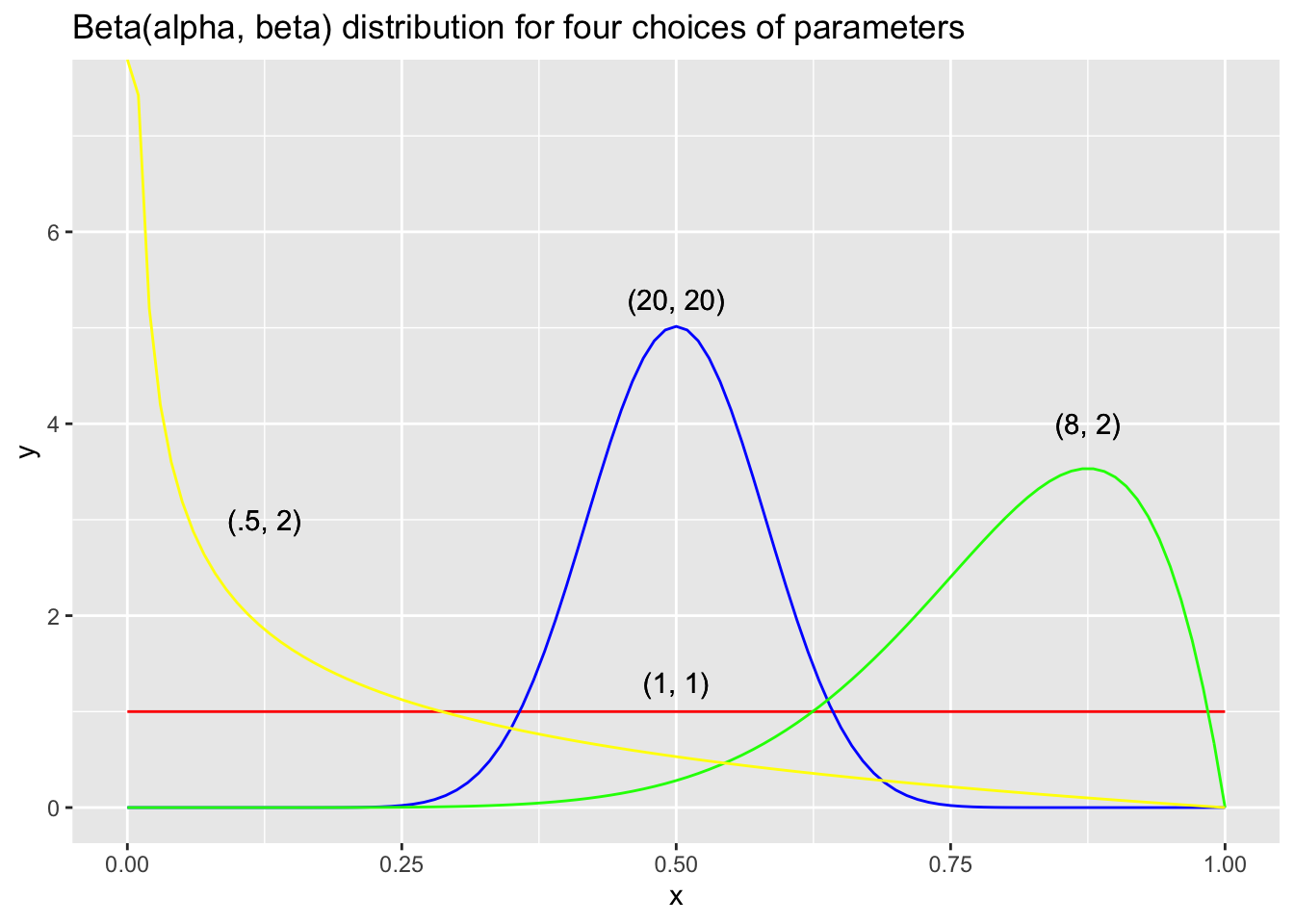
A beta(\(\alpha, \beta\)) random variable has mean \(\frac{\alpha}{\alpha + \beta}\), variance \(\frac{\alpha \beta}{(\alpha + \beta)^2(\alpha + \beta + 1)}\) and mode \(\frac{\alpha - 1}{\alpha + \beta - 2}\) (when \(\alpha > 1\) and \(\beta > 1\)). Together, these facts say that as \(\alpha\) and \(\beta\) get larger, the pdf of a beta random variable concentrates with a peak of \(\frac{\alpha - 1}{\alpha + \beta - 2}\), but with mean closer to 1/2. This is consistent with left skewness when \(\alpha > \beta\) and right skewness when \(\alpha < \beta\). Let’s examine some plots.
Suppose we have a beta prior for \(\theta\) with parameters \(\alpha\) and \(\beta\), and we collect \(j\) heads and \(k\) tails (in some order) out of our \(n = j + k\) trials. We can compute the posterior probability of \(\theta\) given the data as follows. \[ \begin{aligned} p(\theta|D) &= \frac{p(D|\theta) p(\theta)}{p(D)}\\ &= \frac{\theta^j (1 - \theta)^{k} \times p(\theta)}{p(D)}\\ &= \frac{\theta^{j + \alpha - 1} (1 - \theta)^{k + \beta - 1}}{B(\alpha, \beta) p(D)} \end{aligned} \] As before, we ignore the constants in the denominator, and we focus on the form of the pdf. In this case we can see it must be beta with parameters \(\alpha + j\) and \(\beta + k\). This is a very nice relationship. It says that if you have a beta prior and collect data, for each head you obtain, you add one to the \(\alpha\) parameter, and for each tail you obtain, you add one to the \(\beta\) parameter. The result will be a posterior distribution whose standard deviation is getting smaller, and the mean is approaching some value.
Example Suppose \(\theta\) has a prior of \(\alpha = 2\) and \(\beta = 2\). You collect 20 data points and obtain 13 heads and 7 tails. Find the posterior distribution of \(\theta\). Use the posterior to find an interval that contains 95% of the probability mass of the posterior distribution of \(\theta\).
From above, the posterior is \(\alpha = 15\) and \(\beta = 9\). A plot of the pdf looks like this.
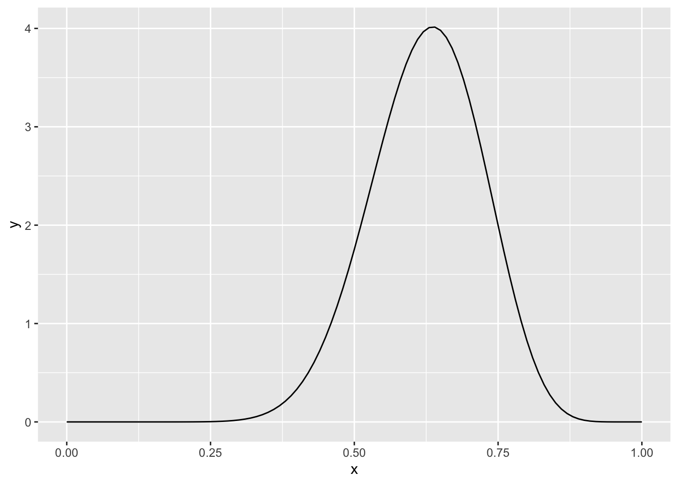 We can find an interval which contains 95% of the probability mass of the posterior by using
 qbeta:
## [1] 0.4273440 0.8029236The solution is \([0.427344, .8029236]\).
16.2.2 Technical Discussions
This sub-section requires more R than the rest of this chapter. Often, when setting a prior, we may have an idea about the central tendency of \(\theta\) and the standard deviation of \(\theta\), and we will need to convert those to \(\alpha\) and \(\beta\) values. This can be done in the following way.
Example Find \(\alpha\) and \(\beta\) so that the mode of a beta random variable with parameters \(\alpha\) and \(\beta\) are 0.7 and 0.02.
We have two equations in two unknowns that we need to solve:
\[
\begin{aligned}
0.7 &= \frac{\alpha - 1}{\alpha + \beta - 2}\\
0.02 &= \sqrt{\frac{\alpha \beta}{(\alpha + \beta)^2(\alpha + \beta + 1)}}
\end{aligned}
\]
A general technique for doing this is to create a non-negative function that has a zero at the solution, then minimize said function using nlm.
We create a function that has a single arugment, x, that we assume is a vector of length 2. We store the first value in alpha and the second value in beta, and write a function that is 0 exactly when the two equations are solved. It is simpler to square both sides of the second equation.
We call nlm using the first parameter f_loss, the function that we are minimizing, and the second parameter p which is a vector of initial values that are a guess for what alpha and beta might be. Note that they do not necessarily have to be very close to correct, as this example shows!
f_loss <- function(x) {
  alpha <- x[1]
  beta <- x[2]
  (0.7 - (alpha - 1)/(alpha + beta - 1))^2 +
  (0.0004 - (alpha * beta)/((alpha + beta)^2 * (alpha + beta + 1)))^2
}
nlm(f_loss, c(10, 20))
## $minimum
## [1] 2.420537e-10
##
## $estimate
## [1] 353.0044 150.8579
##
## $gradient
## [1] 1.799736e-09 -4.290125e-09
##
## $code
## [1] 1
##
## $iterations
## [1] 38We see that the values of alpha and beta that provide a mode of 0.7 and standard deviation of 0.02 are \(\alpha = 353\) and \(\beta = 151\), rounded to the nearest integer.
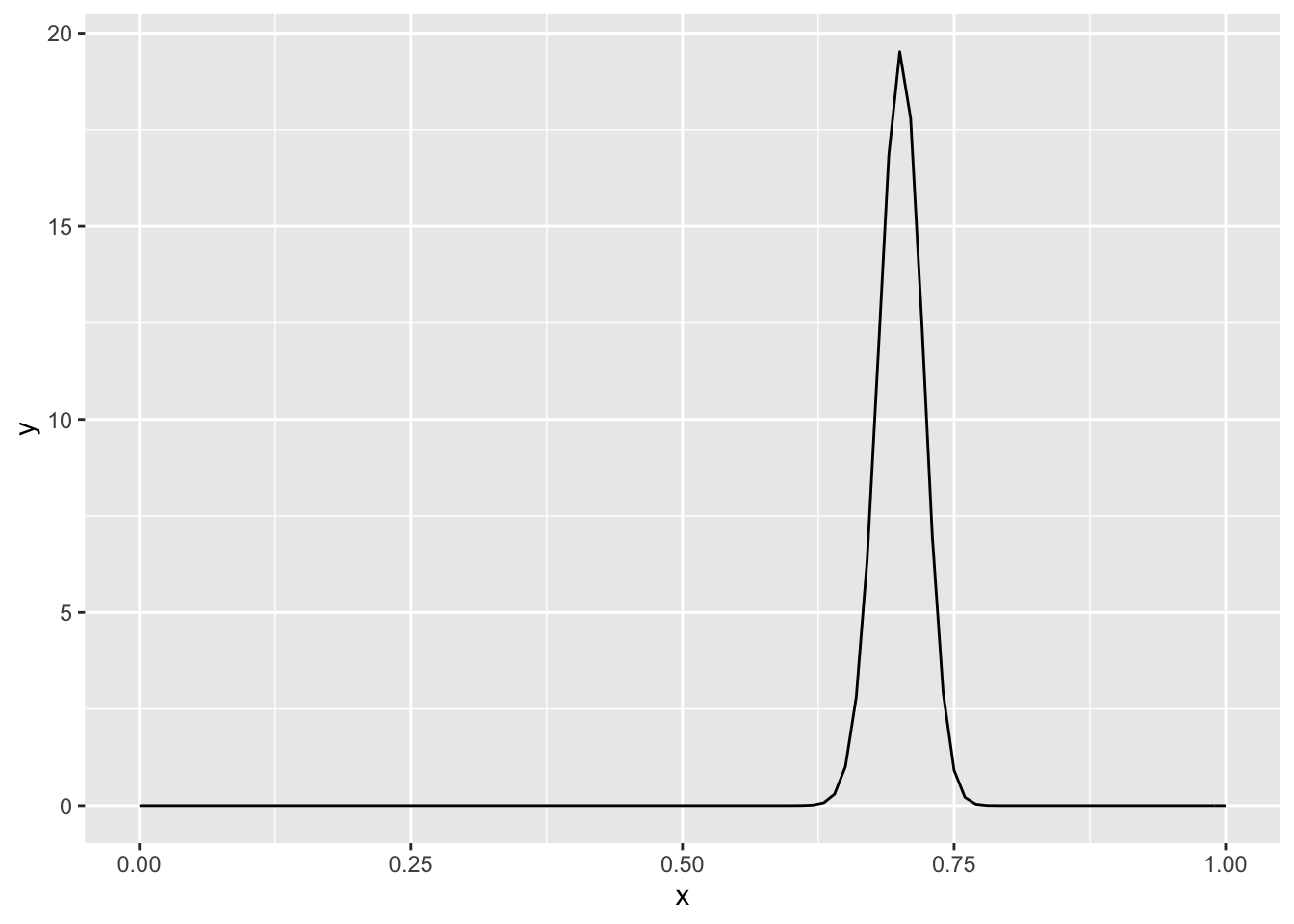 Based on the plot, the mode seems to be about 0.7, as desired, and the standard deviation is approximately 0.02, as estimated below.
## [1] 0.0201842916.2.3 A non-beta prior
In this section, we discuss how we can proceed if we have a non-beta prior for \(\theta\). We could, for example, have a coin that we have reason to believe turns up about 25% heads or 25% tails, but we aren’t sure which. A reasonable prior might be a mixture of scaled and shifted beta random variables, as below.
theta_prior <- function(x) {
  dbeta(2 * x, 10, 10)/2 + dbeta(2 * (x - .5) , 10, 10)/2
}
ggplot(data.frame(x = c(0, 1)), aes(x)) +
  stat_function(fun = theta_prior)
Let’s look at some likelihood ratios for \(\theta\) with this prior. We are saying that we believe that \(\theta = 0.75\) is theta_prior(0.75)/theta_prior(0.6), or about 56, times more likely than \(\theta = 0.6\), and theta_prior(0.75)/theta_prior(0.55), or about 10000 times as likely as \(\theta = 0.55\). This may reflect a well-reasoned belief, but it may also be an undesirable artifact of the model for the prior.
Moreover, in the above prior, the likelihood that \(\theta\) is 0.5 is zero, as is the likelihood that \(\theta\) is 0 or 1. If we wish to make those values less unlikely in our prior belief, we could add some small constant to all of the \(\theta\) values; say 0.01. (Note that this would make the integral of the prior 1.01, so if we wanted to keep it a pdf, we would need to divide by 1.01.)
theta_prior <- function(x) {
dbeta(2 * x, 10, 10)/2 + dbeta(2 * (x - .5) , 10, 10)/2 + .01
}
ggplot(data.frame(x = c(0, 1)), aes(x)) +
stat_function(fun = theta_prior)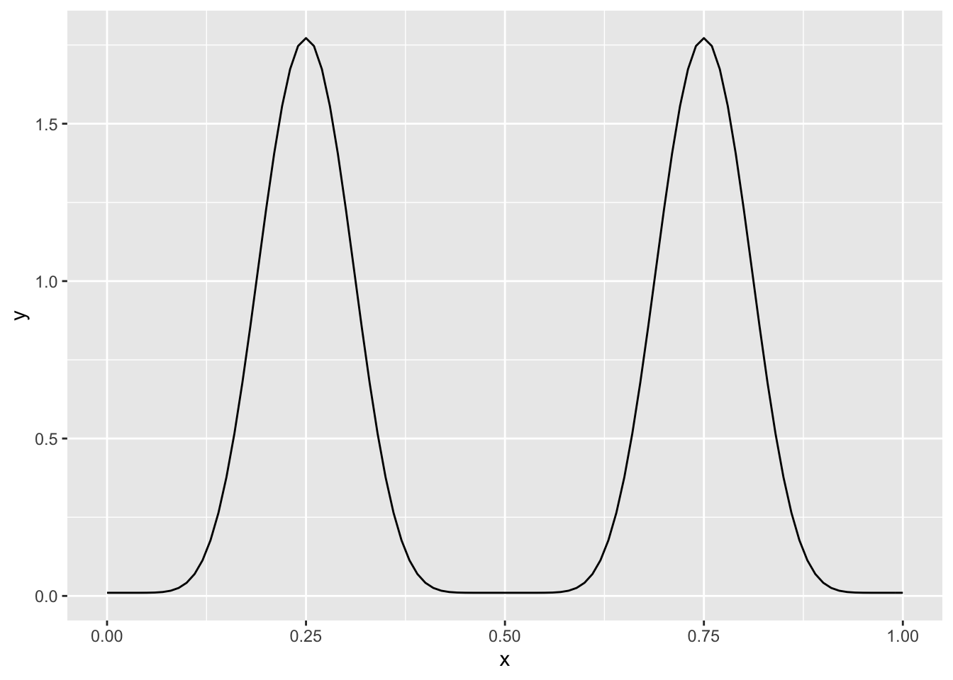 Now the maximum ratio of likelihoods is between \(\theta = 0.75\) and \(\theta = 0.5\), and is about 177. This indicates a belief we have that values outside of the two humps are possible, but much less likely than the values close to 1/4 or 3/4.
Next, suppose that we collect 10 tosses of coins, and we obtain 6 heads and 4 tails in some order. The posterior density is
\[
\begin{aligned}
p(\theta|D)&=\frac{p(D|\theta) p(\theta)}{p(D)}\\
&=C (\theta)^6(1 - \theta)^4 p(\theta)
\end{aligned}
\]
where \(p(\theta) =\)theta_prior(theta) and \(C\) is the normalizing constant. We can compute \(C\) by integrating the rest of the posterior.
theta_posterior_unnormalized <- function(x) {
  x^6 * (1 - x)^4 * theta_prior(x)
}
integrate(f = theta_posterior_unnormalized, lower = 0, upper = 1)
## 0.0002016239 with absolute error < 6.2e-08C <- 1/integrate(f = theta_posterior_unnormalized, lower = 0, upper = 1)$value
theta_posterior <- function(x) {
C * theta_posterior_unnormalized(x)
}Now we can visualize the posterior by plotting it. We plot the prior on the same plot so that we can see how it changed. We also show what would have resulted from a uniform prior on \(\theta\).
ggplot(data.frame(x = c(0, 1)), aes(x)) +
  stat_function(fun = theta_prior) +
  stat_function(fun = theta_posterior, color = "red") +
  stat_function(fun = ~dbeta(.x, 7, 5), color = "green")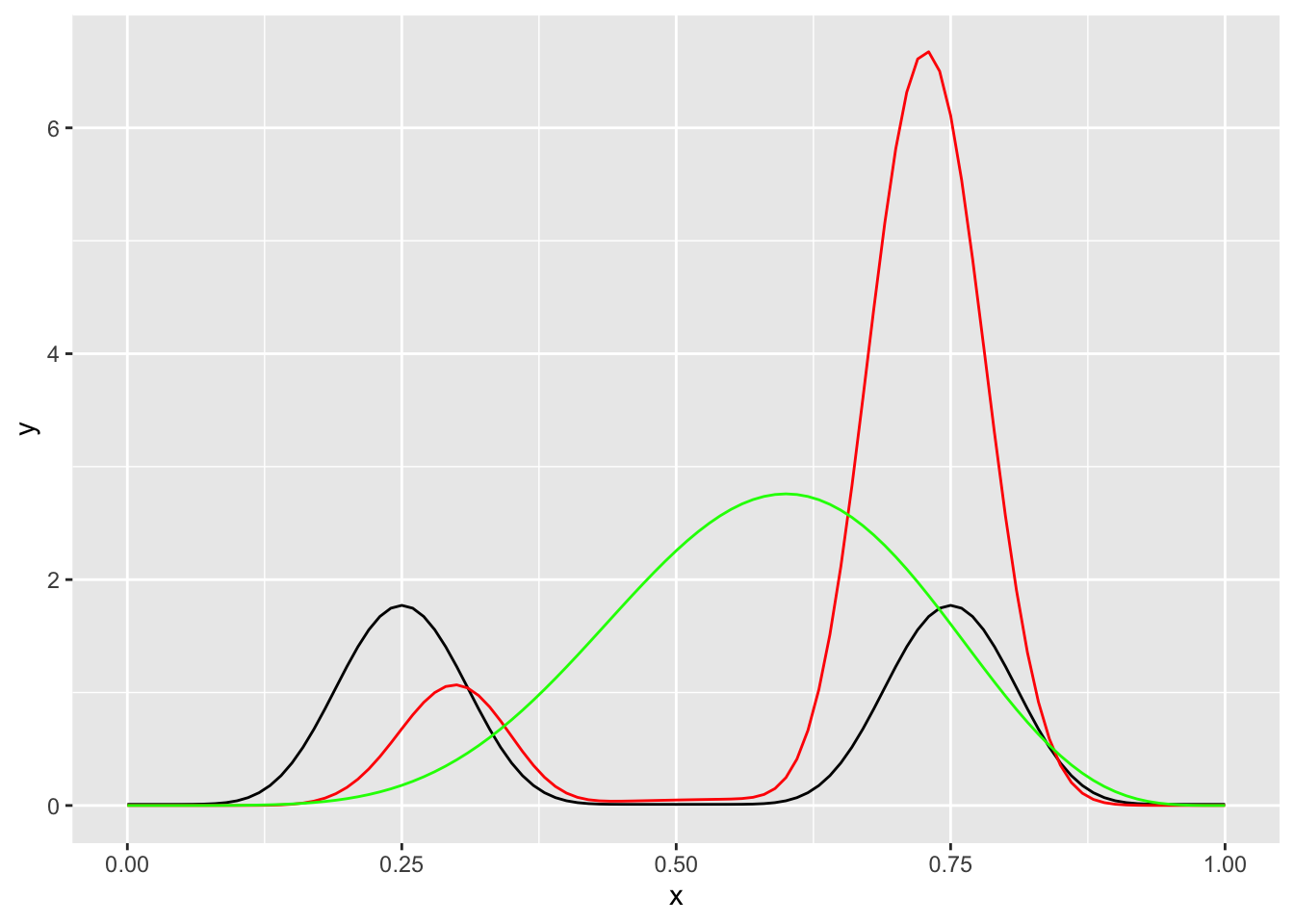
Note what happens, though, if we toss the coin 100 times and obtain 50 heads. This is an indication that perhaps our our prior belief that the coin was heads either 25% or 75% of the time was not correct, and that \(\theta\) is closer to 0.5 than what we had initially thought.
theta_posterior_unnormalized <- function(x) {
  x^50 * (1 - x)^50 * theta_prior(x)
}
integrate(f = theta_posterior_unnormalized, lower = 0, upper = 1)
## 1.588798e-33 with absolute error < 3.4e-34C <- 1/integrate(f = theta_posterior_unnormalized, lower = 0, upper = 1)$value
theta_posterior <- function(x) {
C * theta_posterior_unnormalized(x)
}ggplot(data.frame(x = c(0, 1)), aes(x)) +
stat_function(fun = theta_prior) +
stat_function(fun = theta_posterior, color = "red")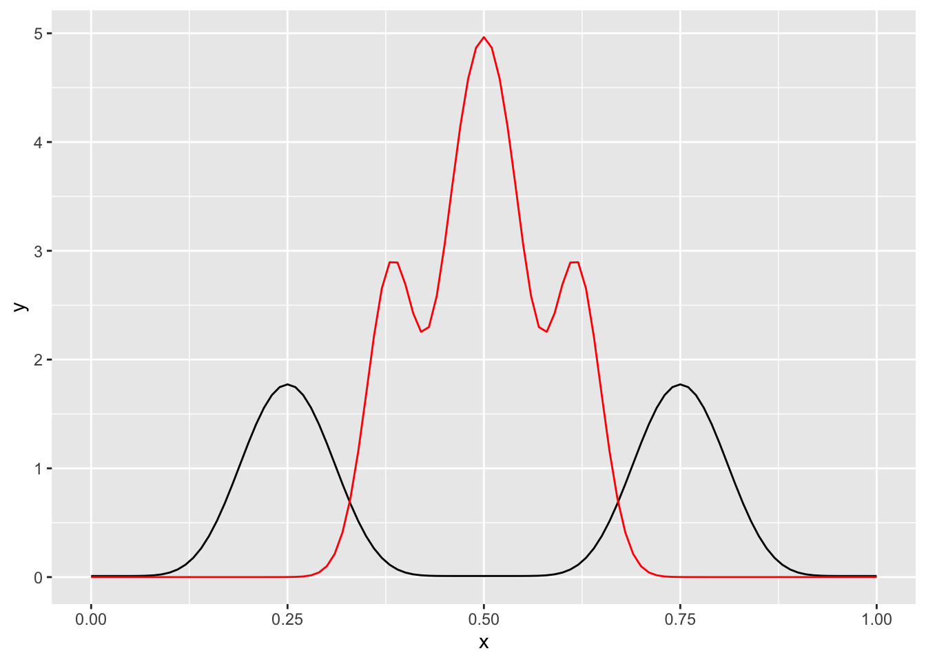
16.3 Priors and Posteriors for Means
In this section we suppose that we are sampling from a normal population with unknown mean \(\mu\) and known standard deviation \(\sigma\). We assume that we have some prior notion of what the mean is, which we can express as a normal random variable with mean \(M\) and standard deviation \(\sigma_2\). If we collect a single data point, \(x\), how can we update our estimate for \(\mu\) to a posterior distribution given the data? The procedure is the same as in the case of Bernoulli trials, but the algebra is a bit more complicated.
We have the following computation. You are asked to fill in the algebraic details and justifications in Exercise ??.
\[
\begin{aligned}
p(\mu|D) &= p(D|\mu)p(\mu)\\
&= \frac{1}{\sqrt{2\pi} \sigma} e^{-(x - \mu)^2/2\sigma^2} \frac{1}{\sqrt{2\pi} \sigma_2} e^{-(\mu - M)^2/2\sigma_2^2}\\
&= Ce^{(2x\mu - \mu^2)/(2\sigma^2) + (-\mu^2 + 2\mu M)/(2\sigma_2^2)}\\
&=C e^{-\frac{1}{2\sigma^2 \sigma_2^2} (\mu^2(\sigma_2^2 \sigma^2) - 2\mu (x\sigma_2^2 + M \sigma^2)}\\
&=C e^{-\frac{\sigma^2 + \sigma_2^2}{2\sigma^2\sigma_2^2}(\mu^2 - 2\frac{x\sigma_2^2 + M\sigma^2}{\sigma^2 + \sigma_2^2}\mu)}\\
&=C^\prime e^{-(\mu - \frac{x\sigma_2^2 + M\sigma^2}{\sigma_2^2+ \sigma^2})}
\end{aligned}
\]
The above computation shows that the posterior distribution of \(\mu\) given the data is normal with mean \(\frac{x\sigma_2^2 + M\sigma^2}{\sigma_2^2+ \sigma^2}\) and standard deviation \(\sqrt{\frac{\sigma_2^2 \sigma^2}{\sigma_2^2 + \sigma^2}}\).
It can be easier to remember and understand this relationship in terms of precision. The precision of a normal random variable is given by one over the variance. Recall that the prior for \(\mu\) is normal with mean \(M\) and standard deviation \(\sigma_2\). Therefore, the prior had mean \(M\) and precision \(\tau_2 = 1/\sigma_2^2\). The underlying distribution has mean \(\mu\) and precision \(\tau_1 = 1/\sigma^2\). Making these substitions yields the mean of the posterior is \(\frac{x/\tau_2 + M/\tau_1}{1/\tau_2 + 1/\tau} = x \frac{\tau_1}{\tau_1 + \tau_2} + M \frac{\tau_2}{\tau_1 + \tau_2}.\) That is, the new mean is a weighted average of the prior mean and the new data, where the weight is determined by the precision. The formula for the precision of the posterior is \(\tau_{post} = \tau_1 + \tau_2\), the sum of the precision in the prior and the precision of the distribution.
If we take a random sample \(x_1, \ldots, x_n\) from the distribution, then we can sequentially update the posterior based on each new data point. Since the precisions add each time, we get \(\tau_{post} = n \tau_1 + \tau_2\). You will show in Exercise ?? that the mean of the posterior is given by \(\mu_{post} = \overline{x} \frac{n \tau_1}{n \tau_1 + \tau_2} + M \frac {\tau_2}{n \tau_1 + \tau_2}\), which is again a weighted sum of the mean of the data and the prior mean, where the weight is related to the precisions.
Example Let’s consider again the mean body temperature of healthy adults, which is in UsingR::normtemp. It might be reasonable to assign a normal prior with mean 98.6 and precision \(1/.1^2\), which corresponds to a standard deviation of \(0.1\). We assume that the true standard deviation of mean temperatures of healthy adults is \(0.75\), so that the precision is 16/9. (Better would be to admit that the standard deviation is unknown, but that is beyond the scope of what we are doing in this chapter.) We collect 130 data points, and we compute the posterior estimate of \(\mu\) to be normal with mean \(\frac{98.6 (100) + 98.25 (130) 16/9}{100 + 130 (16/9)} = 98.3557\) and precision \(100 + 130 (16/9) = 331.111\).
Let’s plot the prior and the posterior.
prior_mean <- function(x) {
dnorm(x, 98.6, .1)
}
posterior_mean <- function(x) {
dnorm(x, 98.3557, 1/sqrt(331.111))
}
ggplot(data.frame(x = c(98, 99)), aes(x)) +
stat_function(fun = prior_mean) +
stat_function(fun = posterior_mean, color = "red")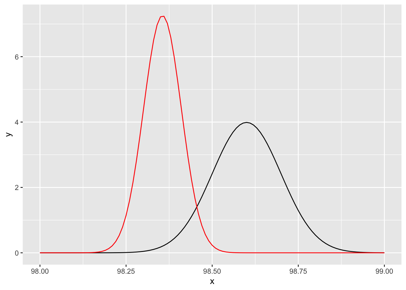 We could compute a 95% credible interval for the mean temperature of healthy adults based on this posterior by using
 qnorm.
## [1] 98.24799 98.46341We see that the 95% credible interval is \([98.248, 98.463]\). So, even with a relatively strong prior that the mean is centered at 98.6, the data indicates otherwise. Notice also that the posterior assigns relatively high likelihood to values such as 98.23, which were considered very unlikely in the prior. This is an indication that our prior is influencing the posterior, which is how it was designed, but if the prior was meant to be a vague prior that didn’t include much information, it may be that we haven’t succeeded in making the prior vague enough.
Let’s see what would have happened had we chosen a less precise prior, as our reasons for choosing 98.6 degrees are (at least in the case of the authors) purely anecdotal, and we thought we were choosing a vague prior. We can be sure that the mean temperature of healthy adults is greater than 96 and less than 101, so perhaps a better standard deviation would be 5/4. A two standard deviation interval around 98.6 then contains all possible values of the true mean. The associated precision is 16/25, and the posterior mean and standard deviation after collecting the same data would have been \(\mu = 98.25096\) and the precision would be 231.7511. An associated 95% credible interval would be \([98.12221, 98.37971]\), as given by the following R command.
## [1] 98.12221 98.37971