Chapter 14 Transformations of Random Variables

In this chapter, we discuss the theory necessary to find the distribution of a transformation of one or more random variables. While the emphasis of this text is on simulation and approximate techniques, understanding the theory and being able to find exact distributions is important for further study in probability and statistics. For one, it is a part of the common knowledge base that probabilists and statisticians know and use when discussing things. We may need to apply theory to know what types of things to approximate or compute when faced with a new situation. Even if we are only concerned in approximate solutions in known contexts, we can often get much better approximations if we apply some theory to the problem. We will see examples of this below.

14.1 Method of Distribution Functions

One method that is often applicable is to compute the cdf of the transformed random variable, and if required, take the derivative to find the pdf.

Example Let \(X\) be a random variable with pdf given by \(f(x) = 2x\), \(0 \le x \le 1\). Find the pdf of \(Y = 2X\).

First, note that the cdf of \(X\) is \[ F_X(x) = \begin{cases} 0&x < 0\\ x^2 & 0\le x \le 1\\1 &x > 1 \end{cases} \]

To find the cdf of \(Y\), we compute

\[ \begin{aligned} F_Y(y) &= P(Y \le y)\\ &= P(2X \le y) \\ &= P(X \le y/2)\\ &= P_X(y/2) \end{aligned} \] So \[ F_Y(y) =\begin{cases} 0 & y/2 < 0\\ (y/2)^2 & 0 \le y/2 \le 1\\ 1 & y/2 > 1 \end{cases} \] and \[ F_Y(y) = \begin{cases} 0&y < 0\\ y^2/4 & 0\le y \le 2\\1 &y > 2 \end{cases} \]

Taking the derivative, we see that \[ f_Y(y) = \begin{cases} y/2 & 0\le y \le 2\\0 &\text{otherwise} \end{cases} \]

There is a shortcut that can be used, where we don’t have to explicitly compute the cdf.

Example Let \(X\) be a standard normal random variable. Find the pdf of \(Y = X^2\).

If we were to proceed as in the first example, we would be stuck at the very first step of writing down the cdf of \(X\). However, we simply write it as \(F_X(x)\). Then, \[ F_Y(y) = P(Y \le y) = P(X^2 \le y) \] so \[ F_Y(y) = \begin{cases} P(-\sqrt{y} \le X \le \sqrt{y})& y \ge 0\\ 0 & y < 0 \end{cases} \] so \[ F_Y(y) =\begin{cases} F_X(\sqrt{y}) - F_X(\sqrt{y}) &y \ge 0 \\ 0 & y < 0 \end{cases} \]

To find the pdf, we differentiate, using the chain rule and the fact that \(F_X^\prime(x) = f_X(x)\).

\[ f_Y(y) = f_X(\sqrt{y}) 1/2 (y^{-1/2}) + f_X(-\sqrt{y}) (1/2 y^{-1/2}) \qquad y \ge 0 \]

Up to this point, the above would be a general formula for any rv \(X\) defined on the line. Now, we can use the fact that \(f_X\) is symmetric, so \(f_X(x) = f_X(-x)\) to simplify

\[ f_Y(y) = f_X(\sqrt{y}) y^{-1/2} = \frac {1}{\sqrt{2\pi y}} e^{-y/2} \qquad y \ge 0. \]

This random variable has a name: it is a \(\chi\)-squared random variable with one degree of freedom. Let’s check our work with a simulation!

sample_x <- rnorm(10000)  #get a sample from X
sample_y <-sample_x^2 #apply the transformation
hist(sample_y, probability = T)
curve(1/sqrt(2 * pi * x) * exp(-x/2), add = T, col = "blue")

## Warning in sqrt(2 * pi * x): NaNs produced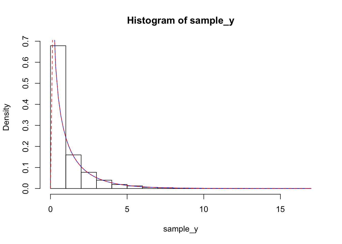

curve(dchisq(x, 1), add = T, col = "red", lty = 2)

We can also use this technique to find the distribution of a combination of two random variables.

Example Let \(X\) and \(Y\) be independent uniform random variables on the interval \([0, 1]\). Find the pdf of \(U = X + Y\).

Since \(X\) and \(Y\) are independent uniform rvs, the joint pdf of \(X\) and \(Y\) is given by \[ f(x, y) = \begin{cases} 1 & 0\le x, y \le 1\\0 &\text{otherwise} \end{cases} \] We compute \[ \begin{aligned} F_U(u) &= P(U \le u)\\ &=P(X + Y \le u) \end{aligned} \]

INSERT PICTURES HERE When \(u < 0\) we get 0, and when \(u > 2\) we get 1. When \(0\le u\le 1\), we get \[ \begin{aligned} P(X + Y \le u) &= \int_{0}^u \int_0^{u - x} 1\, dydx \\ &=\int_0^u u - x\, dx\\ &= u^2 - u^2/2 = u^2/2 \end{aligned} \] Note that since the distribution is uniform we could have just computed the area of the triangle in figure ??. That is not how it is done in general.

When \(1 \le u \le 2\), we get \[ \begin{aligned} P(X + Y \le u) &= 1 - P(X+Y \ge u) \\ &= 1 - \int_{u-1}^1 \int_{u - x}^1 1\, dy dx\\ &=1 - \int_{u-1}^1 1 + x - u\, dx\\ &=1 - 1/2(u - 2)^2 \end{aligned} \] Taking the derivative gives us

\[ f_U(u) = \begin{cases} u & 0\le u\le 1\\ -u + 2 & 1\le u \le 2\\ 0&\text{otherwise} \end{cases} \]

Let’s again check our computation via simulation.

dat <- replicate(10000, {
  x <- runif(1, 0, 1)
  y <- runif(1, 0, 1)
  x + y
})
hist(dat, probability = T)
curve(x + 0, from = 0, to = 1, add = T, col = "red")
curve(2 - x,from = 1, to = 2, add = T, col = "blue")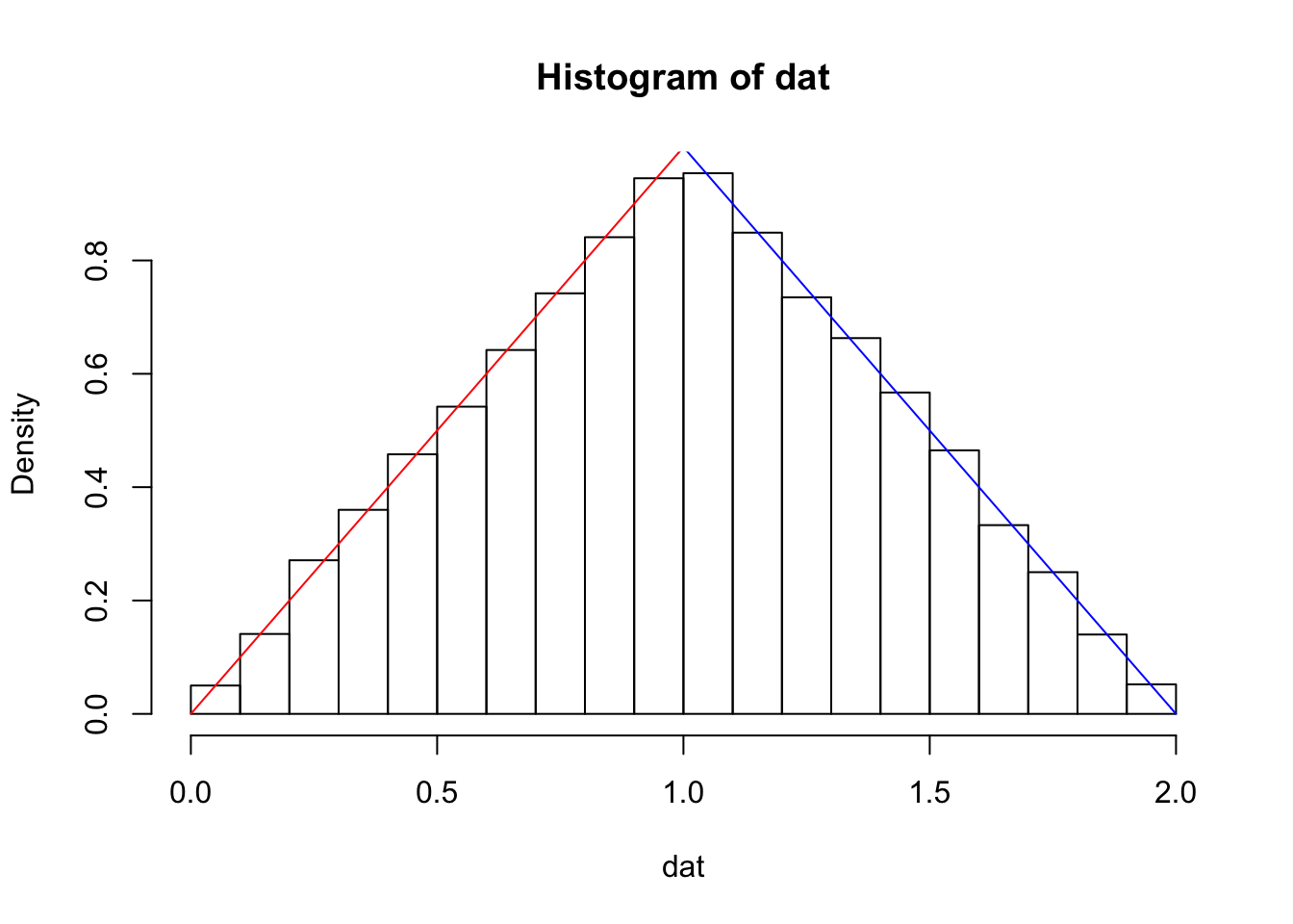

14.2 Moment Generating Functions

Let \(X\) be a random variable, continuous or discrete. We define the moment generating function of \(X\) to be \[ m_X(t) = E[e^{tX}] \] If \(X\) is continuous, this becomes \(\int e^{tx}f(x)\, dx\), and if \(X\) is discrete, this becomes \(\sum e^{tx} p(x)\). There are at least two reasons that we might be interested in moment generating functions. First, as their name implies, mgfs can be used to find the moments of a random variable. Indeed, playing fast and loose with interchanging differentiation and expectation, we have \[ \frac{d}{dt} m_X(t) = E[X e^{tX}] \] which when we evaluate at \(t = 0\) becomes \(E[X]\). So, \(m_X^\prime(0) = E[X]\). More generally, the \(n\)th derivative of \(m_X\) evaluated at zero is the expected value of \(X^n\); \(m^{(n)}(0) = E[X^n]\).

Another important fact about moment generating functions is that if an mgf is defined on a neighborhood of the origin, then the moment generating function determines the distribution of \(X\). From that point of view, knowing a random variable’s mgf gives as much information as the pdf or cdf. Let’s start with some examples of computing moment generating functions.

Example If \(X\) is a discrete random variable with \(P(X = 0) = 1/2\), \(P(X = 2) = 1/3\) and \(P(X = -3) = 1/6\), find the moment generating function of \(X\).

We compute \[ \begin{aligned} E[e^{tX}] &= \sum e^{tx} p(x) = e^{0} p(0) + e^{2t} p(2) + e^{-3t} p(-3) \\ &=1/2 + 1/3 e^{2t} + 1/6 e^{-3t} \end{aligned} \]

Note that we can compute \(E[X] = m_X^\prime(0) = 2e^{2t} (1/3) + -3e^{-3t} (1/6)|_{t = 0} = 2/3 - 1/2 = 1/6\).

Example Let \(X\) be a uniform random variable on the interval \([0, 1]\). Find the moment generating function of \(X\).

We compute for \(t\not= 0\) \[ \begin{aligned} m_X(t) &= \int_0^1 e^{tx}\, dx\\ &=(1/t) e^{tx}|_{x = 0}^1 \\ &= \frac 1t\bigl(e^t - 1\bigr) \end{aligned} \] When \(t = 0\), \(\int f(x)\, dx = 1\) no matter which density function we are using, so we have the following formula for the mgf:

\[ m_X(t) = \begin{cases} \frac 1t(e^t - 1) & t\not= 0\\ 1&t = 0 \end{cases} \]

It can be challenging, in general, to go back and forth between density functions and moment generating functions. One trick for computing mgfs is to re-write the sum or integral that you are trying to compute in terms of something times a probability density or mass function, and then note that the sum or integral of the pmf or pdf is 1. The above two examples did not use that trick, but we present one discrete example and one continuous example below which do use the trick.

Example Let \(X\) be a Poisson random variable with rate \(\lambda\). Find the mgf of \(X\).

We compute:

\[ \begin{aligned} m_X(t) &= \sum_{k = 0}^\infty e^{tk} \lambda^k e^{-\lambda} /k!\\ &= e^{-\lambda} e^{\lambda e^t} \sum_{k = 0}^n (\lambda e^t)^k e^{-\lambda e^t} /k!\\ &= e^{\lambda(e^t - 1)} \end{aligned} \]

where the last line follows from the fact that the rest of the sum is the sum of a Poisson pmf with rate \(\lambda e^t\).

Example Let \(X\) be an exponential random variable with rate \(1\). Find the mgf of \(X\).

We compute, \[ \begin{aligned} m_X(t) &= \int_0^\infty e^{tx} e^{-x}\, dx\\ &= \int_0^\infty e^{-x(1- t)}\, dx\\ &= \frac {1}{1 - t} \int_0^\infty (1 - t) e^{-(1 - t)x}\, dx\\ &= \frac {1}{1 - t} \qquad t < 1 \end{aligned} \]

where the last line follows from the fact that the rest of the integral is the integral of a pdf of an exponential random variable with rate \((1 - t)\), when \(t < 1\).

One nice property of moment generating functions is that they behave nicely with respect to linear combinations of independent random variables. Recall in example ?? above, it was not particularly easy to compute the distribution of \(X + Y\). In many cases, using mgfs makes the computation much simpler.

(#thm:mgf_theorem) Let \(X\) be a random variable with moment generating function \(m_X\). Let \(a\) and \(b\) be real numbers. Then That is, the moment generating function of an affine function of \(X\) can be re-written in terms of the moment generating function of \(X\). Moreover, let \(Y\) be a random variable that is independent of \(X\), which has moment generating function \(m_Y\). Then \[ m_{X + Y}(t) = m_X(t) m_Y(t) \] That is, the moment generating function of the sum of two independent random variables is the product of the two moment generating functions.

The utility of Theorem is the following. Given a transformation of one or more random variables with known mgfs, we can compute the mgf of the transformed random variable. If we recognize the mgf of the transformed random variable, then we know the distribution of the transformed random variable. Let’s look at some examples.

Example Find the mgf of a binomial random variable \(X\) with parameters \(n\) and \(p\).

To do this, we note that \(X = \sum_{i = 1}^n X_i\), where each \(X_i\) is bernoulli with probability of success \(p\). The mgf of each \(X_i\) is given by

\[ \begin{aligned} m_{X_i}(t) &= e^{0} P(X_i = 0) + e^{t} P(X_i = 1)\\ &= p + e^t(1 - p) \end{aligned} \]

Therefore, the mgf of \(X\) is \(\bigl(p + e^t(1 - p)\bigr)^n\).

Example Find the mgf of an exponential random variable \(X\) with rate \(\lambda\).

Using the method of distribution functions, we can see that \(X = \frac 1\lambda Y\), where \(Y\) is exponential with rate 1. (See Exercise ??). Therefore, the mgf of \(X\) is \(m_X(t) = m_{\frac 1\lambda Y}(t) = m_Y(t/\lambda) = \frac 1{1 - t/\lambda} = \frac {\lambda}{\lambda - t}\) when \(t/\lambda < 1\); that is, when \(t < \lambda\).

14.2.1 Method of Moment Generating Functions

Example You will show in Exercise ?? that the moment generating function of a normal random variable with mean \(\mu\) and standard deviation \(\sigma\) is \(m(t) = e^{t\mu} e^{t^2 \sigma^2/2}\). Find the distribution of \(X_1 + X_2\) if \(X_1\) and \(X_2\) are independent normal random variables with means \(\mu_1, \mu_2\) and standard deviations \(\sigma_1, \sigma_2\).

We find the mgf of \(X_1 + X_2\): \[ \begin{aligned} m_{X_1 + X_2}(t) &= m_{X_1}(t) m_{X_2}(t)\\ &=e^{\mu_1 t} e^{\sigma_1^2 t^2/2} e^{\mu_2 t} e^{\sigma_2^2 t^2/2}\\ &=e^{(\mu_1 + \mu_2)t} e^{(\sigma_1^2 + \sigma_2^2)t^2/2} \end{aligned} \] Therefore, \(X_1 + X_2\) is a normal random variable with mean \(\mu_1 + \mu_2\) and standard deviation \(\sqrt{\sigma_1^2 + \sigma_2^2}\), by matching the form of the computed mgf with that of a normal rv. It follows from a similar argument (or by induction) that if \(X_1, \ldots, X_n\) are iid normal with means \((\mu_1, \ldots, \mu_n)\) and standard deviations \((\sigma_1, \ldots, \sigma_n)\), that \(X = \sum_{i = 1}^n X_i\) is normal with mean \(\sum_{i = 1}^n \mu_i\) and standard deviation \(\sqrt{\sum_{i =1}^n \sigma_i^2}\).

Example You will show in Exerecise ?? that the moment generating function of a gamma random variable with rate \(\lambda\) and shape \(\alpha\) is \((1 - t/\lambda)^{-\alpha}\) in some neighborhood of zero. Use this information to find the distribution of the sum of three independent exponential random variables with rate \(\lambda\).

Writing \(X_1, X_2, X_3\) for the independent exponential rvs, we have, since exponential random variables are gamma random variables with shape parameter 1, \[ \begin{aligned} m_{X_1 + X_2 + X_3}(t) &= m_{X_1}(t) m_{X_2}(t) m_{X_3}(t)\\ &=(1 - t/\lambda)^{-1} (1 - t/\lambda)^{-1} (1 - t/\lambda)^{-1} \\ &= (1 - t/\lambda)^{-3} \end{aligned} \] It follows that the sum of the three independent exponentials with common rate \(\lambda\) is gamma with rate \(\lambda\) and shape 3.

14.3 Central Limit Theorem

In this section, we revisit the central limit theorem and provide a theoretical justification for why it is true. Recall that the Central Limit Theorem says that if \((X_i)_{i = 1}^\infty\) are iid random variables with mean \(\mu\) and standard deviation \(\sigma\), that \[ \frac{\overline{X} - \mu}{\sigma/\sqrt{n}} \to Z \] where \(Z\) is a standard normal random variable. In Section ?? we gave some evidence via simulations that the Central Limit Theorem is true. Now we look to provide theoretical evidence that it is true.

We begin with the case that \(X_1, \ldots, X_n\) are scaled; that is, each \(X_i\) has mean 0 and standard deviation 1. We need to show that \[ \sqrt{n}\overline{X} \to Z \] where \(Z\) is standard normal. For our proof, we need to make an additional assumption that the common moment generating function of \(X_1, \ldots\) exists and is defined on a common neighborhood of 0. We use, without proof, the fact that if \(Y_n\) is a sequence of random variables with mgf \(m_{Y_n}\) and \(Y\) is a random variable with mgf \(M_Y(t)\), and if \(m_{Y_n}(t) \to M_Y(t)\) on some interval around \(0\), then the cdf of \(Y_n\) converges to the cdf of \(Y\).

With the above set-up, it remains to show that the moment generating function of \(\sqrt{n}\overline{X} = \frac{1}{\sqrt{n}} \sum_{i = 1}^n X_i\), which we denote by \(m_n(t)\), converges pointwise to \(e^{t^2/2}\), the mgf of a standard normal rv. Let \(m(t)\) be the common mgf of the \(X_i\). Note that, by our assumption on the mean and standard deviation of \(X_i\), the Taylor expansion with remainder of the mgf is given by \(m(t) = 1 + t^2/2 + R(t)\), where \(R(t) \le C |t|^{3}\).

In our first computation, we ignore the remainder so that the idea is clear. This is the key computation to understanding why the Central Limit Theorem is true, based on this approach! \[ \begin{aligned} m_n(t) &= \bigl(m(t/\sqrt{n})\bigr)^n\\ &= \bigl(1 + (t/\sqrt{n})^2/2 + R(t/\sqrt{n})\bigr)^n\\ &\approx (1 + t^2/(2n)\bigr)^n\\ &\to e^{t^2/2} \qquad \text{as } n \to \infty \end{aligned} \] where the last line follows from \((1 + a/n)^n \to e^a\) as \(n\to\infty\).

\[ \begin{aligned} m_n(t) &= \bigl(m(t/\sqrt{n})\bigr)^n\\ &= (1 + t^2/(2n) + R(t/\sqrt{n})\bigr)^n\\ &\to e^{t^2/2} \qquad \text{as } n \to \infty \end{aligned} \]

The last line now follows from the fact that \((1 + a/n + b/n^{3/2})^n \to e^a\), as well, which can be seen by taking the log and applying L’Hopitals Rule. In Exercise ??, a finish to the argument along these lines is given. We need to show the following. If \(X_1, \ldots, X_n\) are iid random variables with mean \(\mu\) and standard deviation \(\sigma\), and \(Y_i = (X_i - \mu)/\sigma\), then \[ \frac {1}{\sqrt{n}} \sum_{i = 1}^n Y_i \to Z. \] from the argument above. Substituting back in \(Y_i = (X_i - \mu)/\sigma\) and doing some algebra yields the form of the Central Limit Theorem stated above.

14.4 Universality of the uniform

In this section, we discuss that the uniform random variable can be used to generate all uni-variate random variables. For simplicity, we assume that we have a continuous random variable \(X\) whose pdf is strictly positive on some interval \([a, b]\) and zero elsewhere. In this case, the cdf of \(X\) is strictly increasing between \(a\) and \(b\), therefore invertible, and there exists a function \(g:[0,1] \to [a,b]\) such that \(g(F_X(x)) = x\) and \(F_X(g(x)) = x\).

Now, we ask: what is the distribution of \(g(U)\), where \(U\) is a uniform random variable defined on \([0, 1]\)? We can use the method of distributions to compute

\[ \begin{aligned} F_{g(U)}(u) &= P(g(U) \le u) \\ &= P(F_X(g(U)) \le F_X(u)) \\ &= P(U \le F_X(u)) \\ &= F_X(u) \end{aligned} \] where the list step is because the cdf of a uniform \([0, 1]\) random variable is given by \(F_U(u) = u\) on the interval \([0, 1]\). Therefore, we have shown that the distribution of \(g(U)\) is the same as \(X\)! This has significant consequences for sampling from random variables. All we need to do is to be able to sample from a uniform random variable and compute the inverse of the cdf of \(X\), then we can sample from \(X\). In the case that \(X\) is discrete or doesn’t satisfy the conditions that we placed on \(X\) in the calculation above, one would need to modify the approach above, but it is still possible.

Example We show how to sample from an exponential random variable with rate 1 using the technique above. We first note that the cdf of an exponential with rate 1 is \(F(x) = 1 - e^{-x}\) \(x \ge 0\). This has inverse function \(g(u) = -\log((u - 1))\). So in order to sample from an exponential random variable, we sample from \([0, 1]\) and apply \(g\).

uniform_sample <- runif(10000, 0, 1)
exponential_sample <- -1 * log(uniform_sample)
hist(exponential_sample, probability = TRUE)
curve(dexp(x), add = T)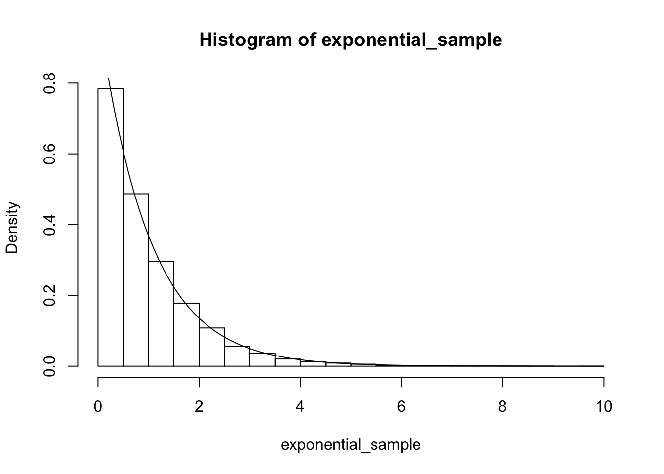

We see that we get a good match.

Example Draw a random sample from a random variable \(X\) with pdf given by \(f(x) = 4x - 4x^3\), \(0\le x \le 1\).

Here the cdf is \(F(x) = 2x^2 - x^4\) when \(0 \le x \le 1\), which is going to be challenging to invert algebraically. However, we can numerically approximate an inverse function using R as follows. We first learned of this method based on the answer by Mike Axiak on stack overflow.

inverse = function (f, lower =  0, upper = 1) {
   function (y) uniroot((function (x) f(x) - y), lower = lower, upper = upper)$root
}

g <- function(x) 2*x^2 - x^4
g_inverse <- inverse(g)
g_inverse(.4)

## [1] 0.4747366

For fixed y, The part of the function inverse given by uniroot((function (x) f(x) - y), lower = lower, upper = upper) gives the value of x such that f(x) = y and is between 0 and 1. In other words, it gives the inverse function evaluated at y. Wrapping that in a function creates a function that is the inverse of the original function.

To use this inside of sampling, it will be convenient to vectorize the return value of the inverse function. But, the return type of g_inverse is a list, so we first have to turn that into a numeric variable.

g_inverse_vectorized <- function(y) sapply(y, g_inverse)
g_inverse_vectorized(c(.1, .2))

## [1] 0.2265170 0.3249192

Now we are ready to go!

uniform_sample <- runif(10000)
x_sample <- g_inverse_vectorized(uniform_sample)
hist(x_sample, probability = TRUE)
curve(4*x - 4*x^3, add = T)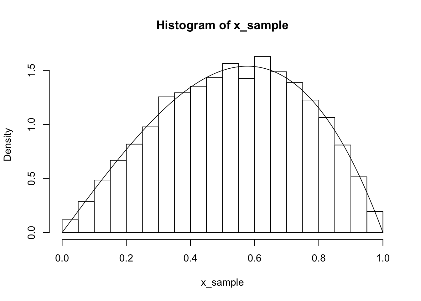

We combine all of the above into a single function which returns a vectorized version of the inverse function of a function supplied.

inverse = function (f, lower = -100, upper = 100) {
   function(y) sapply(y, function (p) 
     uniroot((function (x) f(x) - p), 
             lower = lower, 
             upper = upper)$root
   )
}
g <- function(x) 2 * x^2 - x^4
g_inverse <- inverse(g, lower = 0, upper = 1)
uniform_sample <- runif(10000)
x_sample <- g_inverse(uniform_sample)
hist(x_sample, probability = TRUE)
curve(4*x - 4*x^3, add = T)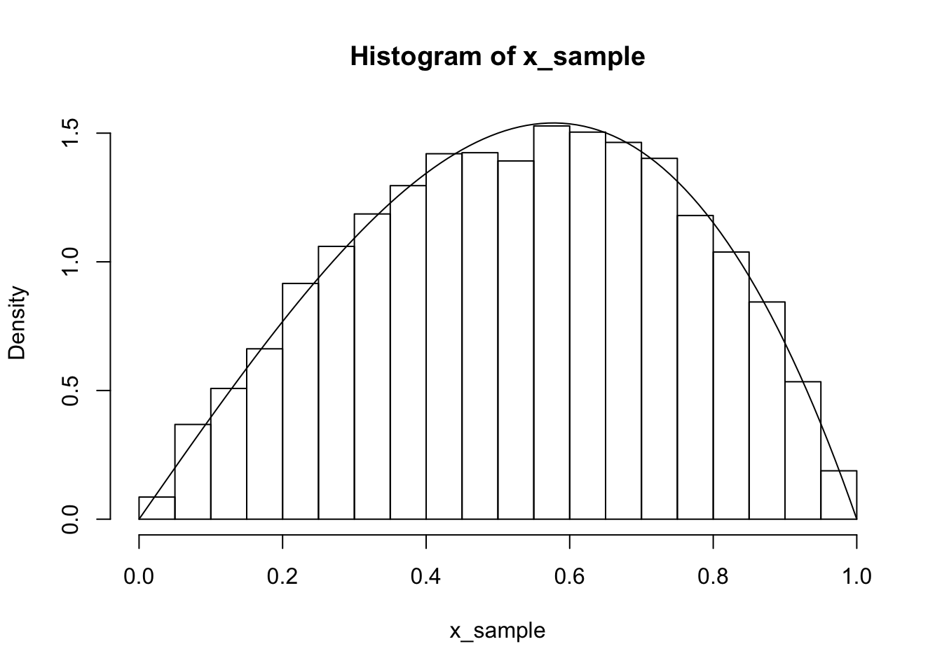

For the majority of this textbook, we try to convince the reader that simulations can be helpful for understanding the theory of probability and for understanding statistics. In the following example, we see that understanding the theory of probability can be very useful when sampling from a distribution!

Example Create a random sample from the joint distribution of \(X\) and \(Y\) when the joint pdf is given by \[ f(x, y) = \begin{cases} 8xy& 0 \le y \le x \le 1\\ 0&\text{otherwise} \end{cases} \]

We begin by computing the marginal distribution of \(X\). \[ \begin{aligned} f(x) &= \int_0^x 8xy \, dy\\ &=4xy^2|0^x\\ &=4x^3 \end{aligned} \] Then, we also need to know the conditional density of \(Y\) given \(X = x_0\). That is given by \(f(x_0, y)/f(x_0) = 8x_0 y/4x_0^3 = 2 x_0^{-2} y\) for \(0 \le y \le x_0\).

Our strategy then is to sample from the marginal of \(X\) to get \(x_0\) and then sample from the conditional density of \(Y\) given \(X = x_0\) to find \(y_0\). The pair \((x_0, y_0)\) is our sample. It helps that in this case, the density of \(X\) is beta(4, 1), which is a built in R function. Unfortunately, the conditional density of \(Y\) given \(X = x_0\) is not a built in R function, this will require us to build custom inverse functions many times. Instead, we do the following trick. Let’s compute the conditional density of \(Y\) divided by \(x_0\) given \(x_0\).

Assuming \(X = x_0\), we have: \[ \begin{aligned} P(\frac {1}{x_0} Y \le y) &= P(Y \le y x_0)\\ &=F(y x_0) \end{aligned} \] where \(F\) is the cdf of \(Y\) given \(X = x_0\). Taking the derivative, we get the density function of \(\frac{1}{x_0} Y\) given \(X = x_0\) is \(2y\) for \(0\le y \le 1\). So, we can sample from that density and then multiply by \(x_0\) to get the sample from \(Y\)!

xs <- rbeta(10000, 4, 1)
ys <- rbeta(10000, 2, 1)
ys <- ys * xs
ggplot(data.frame(x = xs, y = ys), aes(x, y)) +
  geom_density_2d()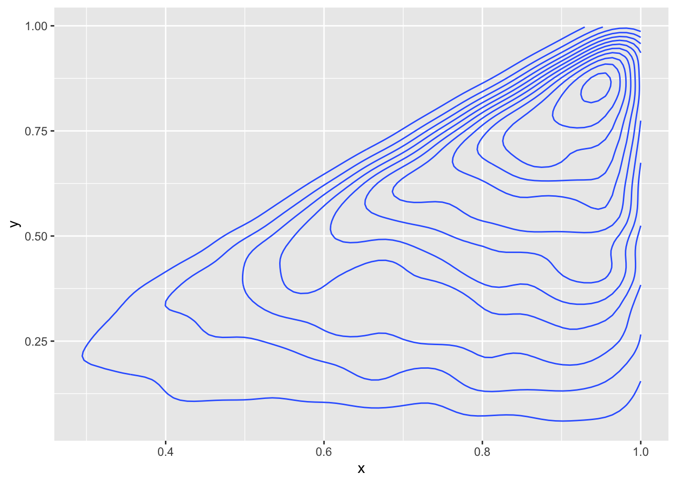

14.5 Order Statistics

In this section we discuss the distribution of order statistics of continuous random variables. Consider a business that receives 50 phone calls per day. Not all of the phone calls can be answered immediately, so some of the customers are placed on hold. The business would reasonably be interested in the maximum hold time of the 50 customers. Or, consider a production process that creates items with a specified strength. Suppose that 10 of the items are going into a crucial piece of a project. The engineer would reasonably be interested in the minimum strength of the items. These are examples of order statistics.

Definition 14.1 Let \(X_1, \ldots, X_n\) be a random sample from a distribution. Let \(X_{(1)}, \ldots, X_{(n)}\) be the random variables sorted from smallest to largest. We call \(X_{(j)}\) the \(j\)th order statistic of the random sample.

We define \(f_{(j)}\) and \(F_{(j)}\) to be the pdf and cdf of the \(j\)th order statistic.

(#thm:max_pdf) Let \(X_1, \ldots, X_n\) be a random sample from a distribution with pdf \(f\) and cdf \(F\). Then, \[ F_{(n)}(x) = \bigl(F(x)\bigr)^n \] and \[ f_{(n)}(x) = n \bigl(F(x)\bigr)^{n-1} f(x) \]

Proof. We use the method of distributions. The event \(X_{(n)} \le x\) is the same as all of the events being less than or equal to \(x\). Therefore, \[ \begin{aligned} F_{(n)}(x) &= P(X_{(n)} \le x)\\ &= P(X_1 \le x, \ldots, X_n \le x)\\ &= \prod_{i = 1}^n P(X_i \le x)\\ &= F(x)^n. \end{aligned} \] The result on pdfs follows by taking the derivative of both sides.

Example Let \(X_1, \ldots, X_n\) be a random sample from a uniform (0, 1) distribution. Find the pdf of \(X_{(n)}\) and recognize it as one that we have studied.

Recall that the cdf of a uniform distribution on the interval \((0, 1)\) is given by \(F(x) = x\) for \(0 \le x \le 1\). Therefore, \[ f_{(n)}(x) = \begin{cases}n x^{n-1}&0 \le x \le 1\\ 0&{\text{otherwise}} \end{cases} \] We see that it is a beta random variable with parameters \(\alpha = n\) and \(\beta = 1\).

Let’s verify this result via simulations when \(n = 3\).

sim_data <- replicate(10000, {
  unif_sample <- runif(3, 0, 1)
  max(unif_sample)
})
plot(density(sim_data), main = "Maximum of uniforms is beta")
curve(dbeta(x, 3, 1), add = T, col = 2)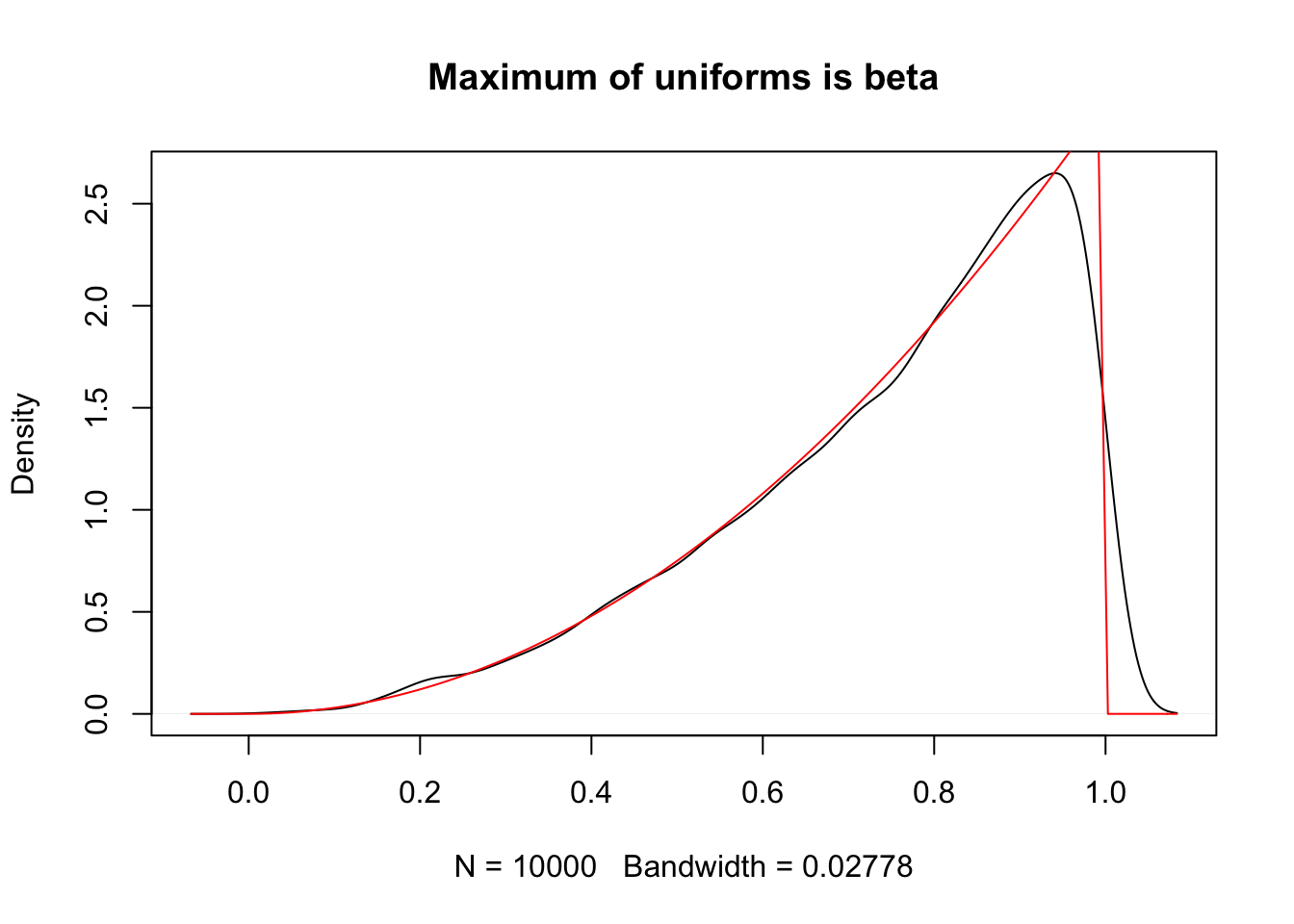

(#thm:min_pdf) Let \(X_1, \ldots, X_n\) be a random sample from a distribution with pdf \(f\) and cdf \(F\). Then, \[ F_{(1)}(x) = 1 - \bigl(1 - F(x)\bigr)^n \] and \[ f_{(n)}(x) = n \bigl(1 - F(x)\bigr)^{n-1} f(x) \]

Proof. We again use the method of distributions. However, the minimum value of a random sample is less than or equal to \(x\) exactly when at least one of the samples is less than \(x\), which is not easy to compute directly. However, if the minimum is greater than \(x\) exactly when all values in the sample are greater than \(x\). Therefore, \[ \begin{aligned} 1 - F_{(n)}(x) &= P(X_{(n)} > x)\\ &=P(X_1 > x, \ldots, X_n > x)\\ &=\bigl(1 - F(x)\bigr)^n. \end{aligned} \] Solving for \(F_{(n)}\) gives the result for cdfs, and taking derivatives gives the result for pdfs.

Example Let \(X_1, \ldots, X_n\) be a random sample from an exponential distribution with rate \(\lambda\). Find the pdf of \(X_{(1)}\), the minimum value.

Recall that the cdf of an exponential is \(F(x) = 1 - e^{-\lambda x}\) for \(x \ge 0\) and the pdf is \(f(x) = \lambda e^{-\lambda x}\). Therefore, \[ f_{(1)}(x) = e^{-(n - 1)\lambda x}e^{-\lambda x} = e^{-n\lambda x}. \] In other words, the minimum of exponentials is again an exponential random variable.

Let’s verify this via simulation when \(n = 4\) and \(\lambda = 1/2\).

sim_data <- replicate(10000, {
  exp_sample <- rexp(4, 1/2)
  min(exp_sample)
})
plot(density(sim_data), main = "Minimum of exponentials is exponential")
curve(dexp(x, 2), add = T, col = 2)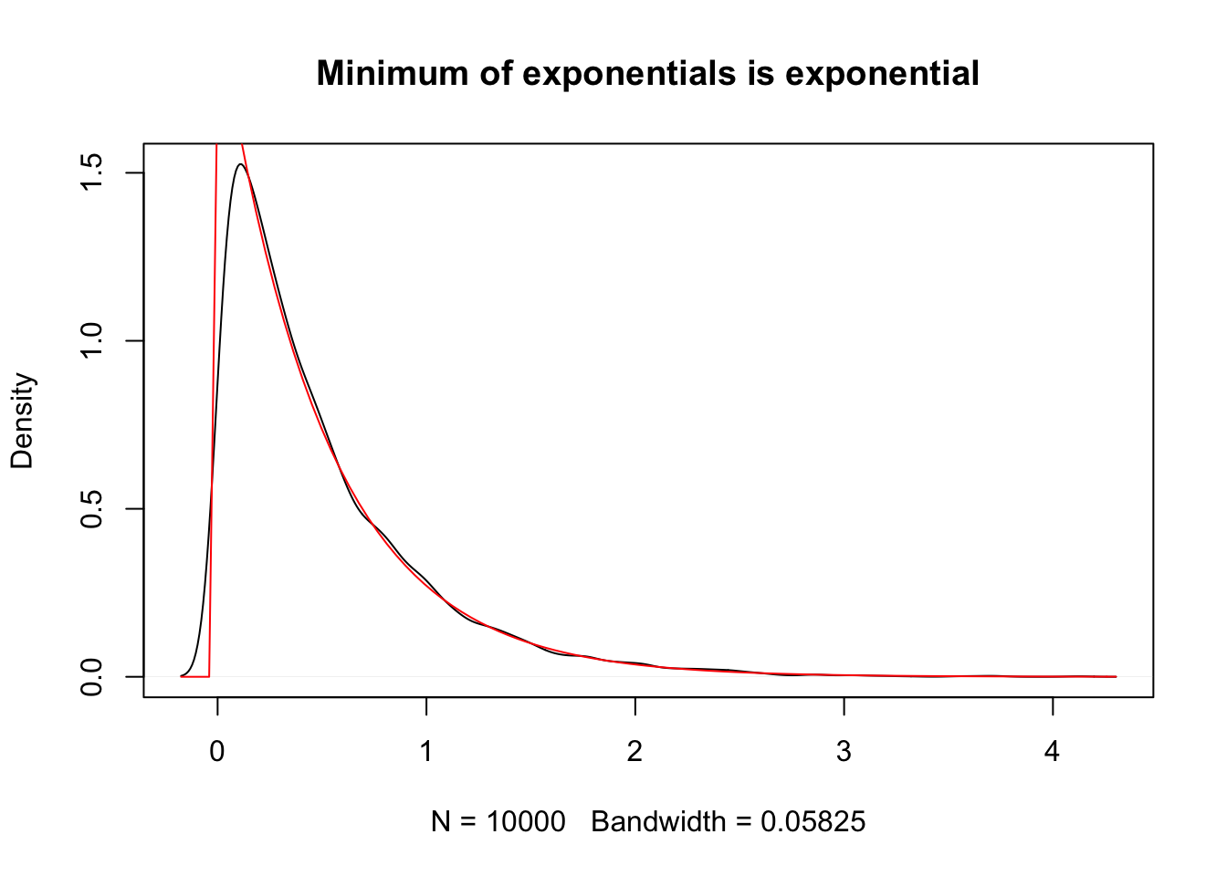

(#thm:order_pdf) Let \(X_1, \ldots, X_n\) be a random sample from a distribution with pdf \(f\) and cdf \(F\). Then, \[ f_{(j)}(x) = \frac{n!}{(n - j)!(n - 1)!} \bigl(F(x)\bigr)^{n - j} \bigl(1 - F(x)\bigr)^{n-1} f(x) \]

Proof. We do not provide a formal proof, but rather an intuitive explanation as to why this is correct. In order for the \(j\)th order statistic to be “about” \(x\), we would need to have \(j - 1\) values less than \(x\), one value about equal to \(x\), and \(n - j\) values greater than \(x\). For each different way of obtaining this arrangement of values, the likelihood is \(\bigl(F(x)\bigr)^{n - j} \bigl(1 - F(x)\bigr)^{n-1} f(x)\). Since there are \(\frac{n!}{(n - j)!(n - 1)!}\) different arrangements possible, we multiply by that value to get the result.

Example Let \(X_1, \ldots, X_{11}\) be a random sample from an exponential distribution with rate 1. The median of an exponential distribution with rate 1 is \(\ln 2\). Compute the pdf of the median \(X_{(6)}\) of the random sample and determine whether \(E[X_{(6)}] = \ln 2\).

The pdf of \(X_{(6)}\) is \[ \begin{aligned} f_{(6)}(x) &= \frac{11!}{5! 5!} (1 - e^{-x})^5 (e^{-x})^5 e^{-x}\\ &= 2772 (1 - e^{-x})^5 e^{-6x} \end{aligned} \] In order to determine \(E[X_{(6)}]\), we need to compute \[ \int_0^\infty 2772 x (1 - e^{-x})^5 e^{-6x}\, dx. \] This is possible via expanding the term \((1 - e^{-x})^5\), multiplying by \(x e^{-6x}\) and using integration by parts on each resulting term. Or, if you are lazy like us, you can trust Wolfram alpha to get the correct answer of \(\frac{20417}{27720}\). At any rate, if you start working on this, you will see that your answer will be rational and not \(\ln 2\).

Let’s verify both the form of the pdf and the estimate of the expected value of \(X_{(6)}\) via simulations. We note that the 6th order statistic is exactly the median value when taking a sample of size 11. We begin by estimating the density function via simulations.

sim_data <- replicate(10000, {
  exp_sample <- rexp(11)
  median(exp_sample)
})
plot(density(sim_data), main = "Density of median of exponentials")
curve(2772 * (1 - exp(-x))^5 * exp(-6*x), add = T, col = 2)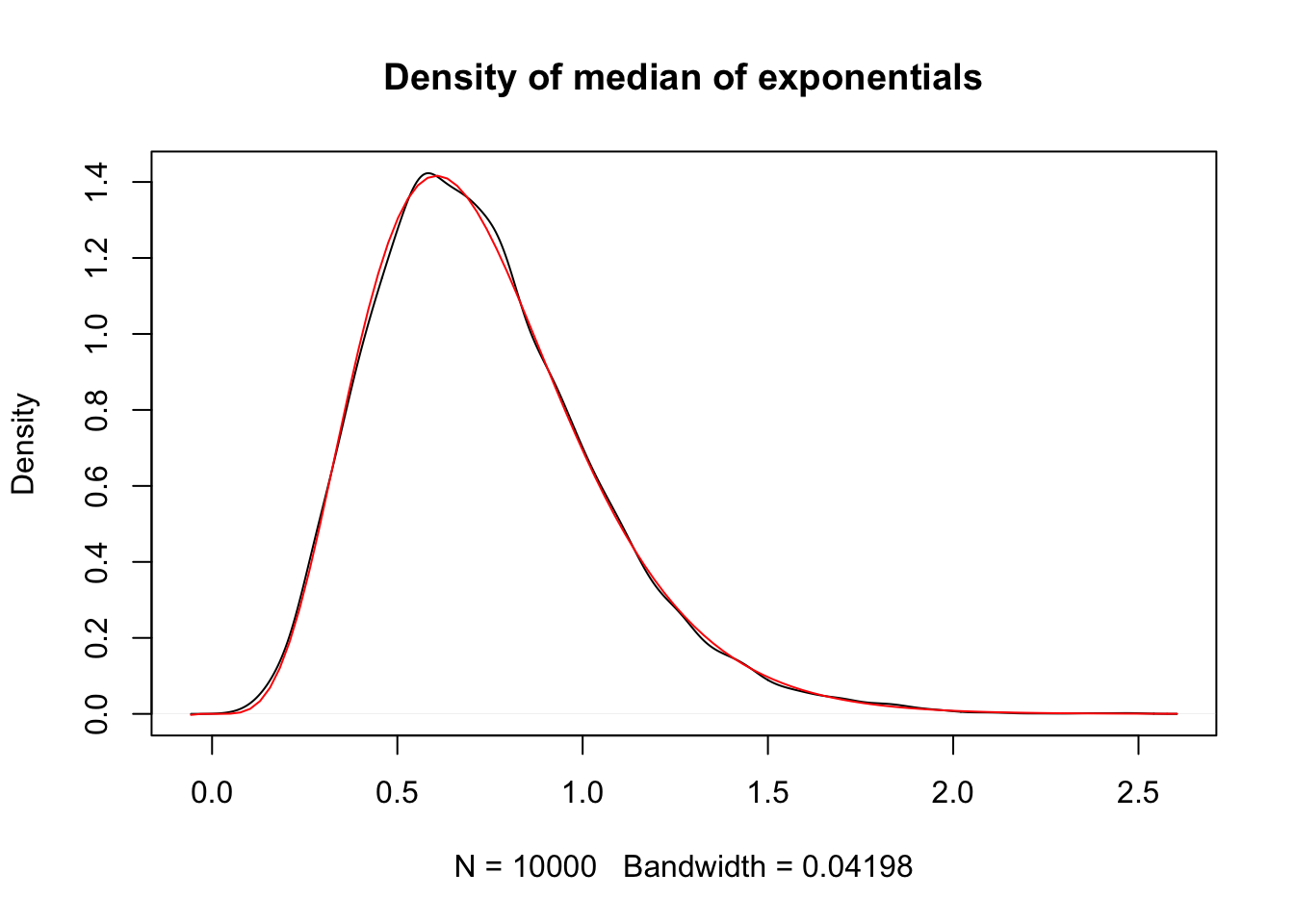

Now, we can use the same sample to estimate the expected value of the median.

mean(sim_data)

## [1] 0.7348512

We see that we get a similar answer to the theoretical result we computed above, which is

20417/27720

## [1] 0.736544

and at an absolute minimum, it is not equal to \(\ln 2 \approx 0.693\). In the language of Chapter @ref(point_estimation), \(X_{(6)}\) is a biased estimator of the median.

14.6 Exercises

Let \(X\) be a uniform random variable on the interval \([-1, 1]\). Find the pdfs of the following random variables.
1. \(X + 1\).
2. \(2X\).
3. \(X^2\)
Let \(X\) be an exponential random variable with rate 1. Let \(\lambda > 0\). Show that \(\lambda X\) is exponential with rate \(1/\lambda\).
Let \(X\) be an exponential random variable with rate \(\lambda\). Find the pdf of \(X^2\).
Let \(X\) and \(Y\) have joint distribution given by \[ f(x, y) = \begin{cases} x + y & 0\le x \le 1, 0 \le y \le 1\\ 0 & \text{otherwise} \end{cases} \]
1. Find the pdf of the random variable \(U = X + Y\).
2. Confirm by taking a random sample from the joint distribution, using it to plot a histogram of a large sample from \(X + Y\), and comparing the histogram to your answer in a.
Let \(X\) and \(Y\) have joint distribution given by \[ f(x, y) = \begin{cases} C xy &1 \le x + y \le 2, 0\le y \le 1\\ 0 & \text{otherwise} \end{cases} \]
1. Find the value of \(C\) that makes this a valid pdf.
2. Find the pdf of the random variable \(U = X + Y\).
3. Confirm by taking a random sample from the joint distribution, using it to plot a histogram of a large sample from \(X + Y\), and comparing the histogram to your answer in b.
Let \(X\) be a discrete random variable such that \(P(X = 0) = 1/3\), \(P(X = 5) = 1/6\), \(P(X = -10) = 1/6\) and \(P(X = 3) = 1/3\). Find the moment generating function of \(X\)/
Let \(X\) be a geometric random variable with probability of success \(p\). Show that the mgf of \(X\) is given by \(m(t) = \frac {p}{1 - (1 - p)e^t}\).
Use the result of the previous exercise to find the mgf of \(\sum_{i = 1}^n X_i\), where the \(X_i\) are iid geometric random variables with probability of success \(p\). Note that this is the number of failures before obtaining n successes, so you will have found the mgf of a negative binomial random variable!
In this exercise, we outline a method for finding the mgf of a normal random variable with mean \(\mu\) and standard deviation \(\sigma\).
1. Find the mgf of a normal random variable with mean \(0\) and standard deivation 1. Hint: \[ \begin{aligned} m(t) &= \frac {1}{\sqrt{2\pi}} \int_{-\infty}^\infty e^{tx} e^{-x^2/2}\\ &= \frac {1}{\sqrt{2\pi}} \int_{-\infty}^\infty e^{-(x^2 - 2t + t^2)/2}e^{t^2/2} \end{aligned} \]
2. Use the method of distributions to show that if \(X\) is a normal random variable with mean \(\mu\) and standard deviation \(\sigma\), then \(X + a\) is normal with mean \(\mu + a\) and standard deviation \(\sigma\).
3. Use the method of distributions to show that if \(X\) is a normal random variable with mean \(\mu\) and standard deviation \(\sigma\), then \(bX\) is normal with mean \(b\mu\) and standard deviation \(b \sigma\).
4. Let \(X\) be a random variable with mean \(\mu\) and sd \(\sigma\). Show that \(X = \sigma Z + \mu\), where \(Z\) is a standard normal rv.
5. Combine the above results to show that the mgf of a normal random variable with mean \(\mu\) and standard deviation \(\sigma\) is \(e^{\mu t + \sigma^2 t^2/2}\).
Show that the mgf of a gamma random variable with rate \(\lambda\) and shape \(\alpha\) is given by \(m(t) = (1 - t/\lambda)^{-\alpha}\) for \(t < \lambda\).
Show that the sum of independent gamma random variables with common rate \(\lambda\) is again gamma. Find the parameters.
Let \(X_1, \ldots, X_n\) be iid exponential random variables with rate \(\lambda\). Show that \(\overline{X}\) is gamma with scale \(n\) and rate \(n \lambda\).
A \(\chi-\)squared random variable with \(\nu\) degrees of freedom is defined to be a gamma random variable with rate 1/2 and shape \(\nu/2\). Show that if \(X_1, \ldots, X_n\) are independent \(\chi-\)squared random variables with degrees of freedom \(\nu_1, \ldots, \nu_n\), then \(\sum_{i = 1}^n X_i\) is \(\chi\)-squared with \(\sum_{i = 1}^n \nu_i\) degrees of freedom.
Show that the sum of independent Poisson random variables \(X_1\) and \(X_2\) with rates \(\lambda_1\) and \(\lambda_2\) is Poisson with rate \(\lambda_1 +\lambda_2\).
Let \(X\) and \(Y\) be independent Posson random variables with common rate \(\lambda\). Find \(P(X = x|X + Y = n)\). (Hint: use definition of conditional probability and then rewrite the numerator as the intersection of two independent events.)
Let \(X\) and \(Y\) be independent geometric random variables with common probability of success \(p\). Find \(P(X = x|X + Y = n)\).
Complete the proof of the Central Limit Theorem given in the text. That is, assuming that we know the Central Limit Theorem is true for mean 0 and standard deviation 1 random variables, show that it is true in general.
Let \(X\) be a random variable with pdf given by \(f(x) = 3x^2\) for \(0\le x \le 1\).
1. Find a function \(g\) such that \(g(U) \sim X\), where \(U\) is a uniform \([0, 1]\) random variable.
2. Use your answer to a to take a random sample from \(X\), plot a histogram, and compare the histogram to the pdf of \(X\).
Let \(X\) be a random variable with pdf given by \(f(x) = \frac{15}{4} \bigl(x^2 - x^4\bigr)\) for \(-1\le x \le 1\).
1. Use the universality of the uniform to sample from \(X\).
2. Plot a histrogram and compare to the pdf of \(X\).