Chapter 13 Joint Distributions of Random Variables
In this chapter, which requires knowledge of multiavariate calculus, we consider the joint distribution of two or more random variables. While much information can be obtained by considering the density functions and distribution functions of random variables indivdually, there are certain instances where we need to know how the variables interact with one another. A first example of this was the correlation between two random variables. In this chapter, though, we will be able to fully specify the dependence (or lack thereof) between two or more random variables. Though our primary focus is on the two random variable continuous case, we start by examining the two random variable discrete case. As in the previous chapters, we continue to emphasize simulation over theory, but this chapter is one of the more theoretical oriented chapters in the textbook.
13.1 Joint probability mass functions
Consider the following scenario. A Halloween candy basket urn contains 8 bags of candy — two bags of Skittles, three Reeses’ peanut butter cups, and three bags of candy corn. You reach in and grab four items of candy at random. Obviously, we don’t care about the candy corn, which are inedible, so we are interested in the distribution of the number of edible candies that we might get out of our 4. With a little bit of counting and work, or simulation, we come up with the following table.
## Warning in kableExtra::add_header_above(., c(` ` = 1, `Number of Reeses` = 4)):
## Please specify format in kable. kableExtra can customize either HTML or LaTeX
## outputs. See https://haozhu233.github.io/kableExtra/ for details.
## Warning in kableExtra::group_rows(., index = c(Skittles = 3)): Please specify
## format in kable. kableExtra can customize either HTML or LaTeX outputs. See
## https://haozhu233.github.io/kableExtra/ for details.| zero | one | two | three | |
|---|---|---|---|---|
| zero | 0 | 3/70 | 9/70 | 3/70 |
| one | 2/70 | 18/70 | 18/70 | 2/70 |
| two | 3/70 | 9/70 | 3/70 | 0 |
Fortunately, we can see that at the very least, we will get at least one piece of good candy! Looking at the table, we can also see that the most likely outcome is that we get two Reeses and one Skittles or one Reeses and one Skittles, each with probability \(18/70\). Not too shabby. If we want to compute the probability of getting exactly one Reeses, then we add up over the various possibilities for the number of bags of Skittles; 3/70 + 18/70 + 9/70 = 30/70.
Definition The marginal distribution of \(X\) is the probability distribution of \(X\), with no reference to other variables. It can be computed by: \[ p_X(x) = \sum_y p(x, y) \] where the sum is over all values of \(y\) such that \(p(x, y) > 0\).
Example We compute the marginal pmf of \(X\), the number of Reeses that we get. We simply add each column to get:
\[
p_X(x) = \begin{cases}
5/70 & x = 0\\
30/70 & x = 1\\
30/70 & x = 2\\
5/70 & x = 3
\end{cases}
\]
Note that in this case, we could have split the candies into Reeses and not Reeses. We would have had 3 Reeses and 5 not Reeses in the bag, from which we drew 4 bags of candy. The distribution of the number of Reeses we obtain is hypergeometric with \(m = 3, n = 5, k = 4\). We check our computation above using dhyper:
## [1] 5 30 30 5Similarly, we can compute \(p_Y(y)\) as \[ p_Y(y) = \begin{cases} 15/70&y = 0\\ 40/70 & y = 1\\ 15/70&y = 2 \end{cases} \] And we could again compare it to hypergeometric with \(m = 2, n = 6, k = 4\) as a check on our work.
Next we imagine a scenario where you ask a friend to look in your bag and see how many bags of Skittles there are. They tell you zero. What is the conditional distribution on the number of bags of Reeses? Well, the probability of getting exactly one bag of Reeses is \[ P(X = 1|Y = 0) = P(X = 1 \cap Y = 0)/P(Y = 0) = \frac{3/70}{15/70} = 1/5 \] More generally, the conditional probability mass function of \(X\) given \(Y\) is defined by
\[ p(x|Y = y) = p(X = x|Y = y) = \frac{p(x, y)}{p_Y(y)}. \]
Example Compute the conditional probability mas function of the number of bags of Reeses \(X\) given that the number of bags of Skittles \(Y\) is zero.
We have \[ p(x|Y = 0) = p(x, 0)/p_Y(0) = \begin{cases} 1/5&x = 0\\ 3/5&x = 1\\ 1/5&x = 2 \end{cases} \] As usual, the probability is zero for all other values of \(x\), including \(x = 0\), which is impossible in this scenario.
13.1.1 Sampling from a joint probability mass function
Before we go on, it would nice if we were able to sample from a joint probability mass function. We can use the base R function sample to do this; we will just need to be careful about keeping track of the indices! We will create a data frame that contains the posible \(X\) and \(Y\) values, as well as their probabilities. Then, we will sample from the data frame with relative likelihood given by the probabilities using the dplyr command sample_n.
data_for_sampling <- data.frame(X = rep(0:3, times = 3), Y = rep(0:2, each = 4))
data_for_sampling <- mutate(data_for_sampling, probs = c(0, 3, 9, 3, 2, 18, 18, 2, 3, 9, 3, 0))
Here is what our data frame looks like:
##    X Y probs
## 1  0 0     0
## 2  1 0     3
## 3  2 0     9
## 4  3 0     3
## 5  0 1     2
## 6  1 1    18
## 7  2 1    18
## 8  3 1     2
## 9  0 2     3
## 10 1 2     9
## 11 2 2     3
## 12 3 2     0
sampled_data <- sample_n(data_for_sampling,
size = 10000,
replace = T,
weight = data_for_sampling$probs)And we can throw away the probability column now.
Once we have a random sample that follows the joint distribution, we can estimate the marginal probability mass functions like this.
## # A tibble: 4 x 3
##       X     n   prob
##   <int> <int>  <dbl>
## 1     0   734 0.0734
## 2     1  4303 0.430
## 3     2  4252 0.425
## 4     3   711 0.0711
We can compare that to the true values that we computed above of 5/70, 30/70, 30/70 and 5/70 and see that we get a very similar answer.
Next, we can find the conditional density of \(X\) given \(Y = 0\). We repeat the exact same procedure as above, but we first filter our data so that \(Y = 0\).
## # A tibble: 3 x 3
##       X     n  prob
##   <int> <int> <dbl>
## 1     1   451 0.208
## 2     2  1294 0.597
## 3     3   421 0.194
Again, we compare with what was computed above; namely, 1/5, 3/5, 1/5.
13.1.2 Expected Values
Now we turn to computing expected values of functions of \(X\) and \(Y\) given the joint probability mass function \(p\). Let \(g(x, y)\) be a real-valued function of two variables. Then, \[ E[g(X, Y)] = \sum g(x, y) p(x, y) \] where the sum is over all pairs \((x, y)\) for which \(p(x, y) \not= 0\).
We will do some exact computations momentarily, but let’s first see how to do this from the random sample that we obtained above.
Example Find the expected number of bags of Reeses candy in the scenario outlined above.
##   expected_x
## 1      1.494
Find the expected value of \(XY\).
##   expected_xy
## 1      1.2791
We define the covariance of \(X\) and \(Y\) to be \[ E[(X - \mu_X) (Y - \mu_Y)] = E[XY] - E[X]E[Y], \] where \(\mu_X\) is the mean of \(X\) and \(\mu_Y\) is the mean of \(Y\). Looking at the first expression, we see that \((X - \mu_X) (Y - \mu_Y)\) is positive exactly when either both \(X\) and \(Y\) are bigger than their means, or when both \(X\) and \(Y\) are less than their means. Therefore, we expect to see a positive covariance if increased values of \(X\) are probabilistically associated with increased values of \(Y\), and we expect to see a negatice covariance when increased values of \(X\) are associated with decreased values of \(Y\).
The correlation of \(X\) and \(Y\) is given by \[ \rho(X, Y) = \frac{E[(X - \mu_X) (Y - \mu_Y)]}{\sigma_X \sigma_Y} \] The correlation is easier to interpret in most cases than the covariance, because the values are between \(-1\) and \(1\). A value of \(\pm 1\) corresponds to a perfect linear relationship between \(X\) and \(Y\), and the larger tha absolute value of the correlation is, the stronger we expect the linear relationship of \(X\) and \(Y\) to be.
We can estimate the covariance and correlation using the built in R functions cov and cor.
## [1] -0.2143238## [1] -0.4437145We should not be surprised to see a negative correlation here, because the more bags of Reeses that I get, the fewer bags of Skittles I would expect to see in my four bags of candy.
We finish by computing one of these by hand. The rest are similar.
\[ \begin{aligned} E[XY] &= \sum xy p(x, y) \\ &= \sum_{x, y \not= 0} xy p(x, y)\\ &= 1 p(1,1) + 2 p(2,1) + 3 p(3,1) + 2p(1,2) + 4 p(2, 2) + 6 p(3, 2)\\ &= 18/70 + 2 * 18/30 + 3 * 2/70 + 2 * 9/70 + 4 * 3/70 + 6 * 0\\ &= 90/70 \end{aligned} \]
13.2 Joint probability density functions
Let \(f(x,y)\) be a function of two variables. We say that \(f\) is a joint probability density function if \(\int \int f(x,y)\, dxdy = 1\) and \(f(x, y) \ge 0\) for all \(x,y\). Given a region in the plane \(R\), the probability that \((x,y)\) is in \(R\) is given by \[ \int_R f(x, y)\, dxdy. \]
Let’s consider an example. Let \[ f(x, y) = \begin{cases} x + y& 0\le x \le 1, 0 \le y \le 1 \\ 0& \mathrm{otherwise} \end{cases} \] We verify that this is a joint pdf by integrating \(f\) over the region \([0, 1] \times [0, 1]\) as follows:
\[ \begin{aligned} \int_0^1 \int_0^1 (x + y)\, dxdy &= \int_0^1 1/2 + y \, dy\\ &= 1/2 + 1/2 y^2|_{y = 0}^{y = 1} \\ &= 1 \end{aligned} \]
and by noting that \(f(x, y) \ge 0\) for all \(x, y\).
13.2.1 Sampling from random variables given (joint) pdf
In this section, we discuss how to sample from random variables given their pdf. In the one-dimensional case, we only considered random variables that had pdf’s with built in R functions that would sample. Unlike the one-dimensional case, however, most two-dimensional distributions do not have built in R root functions. We will develop a technique that allows us to sample from random variables defined by their (joint) pdfs.
13.2.2 One-dimensional case
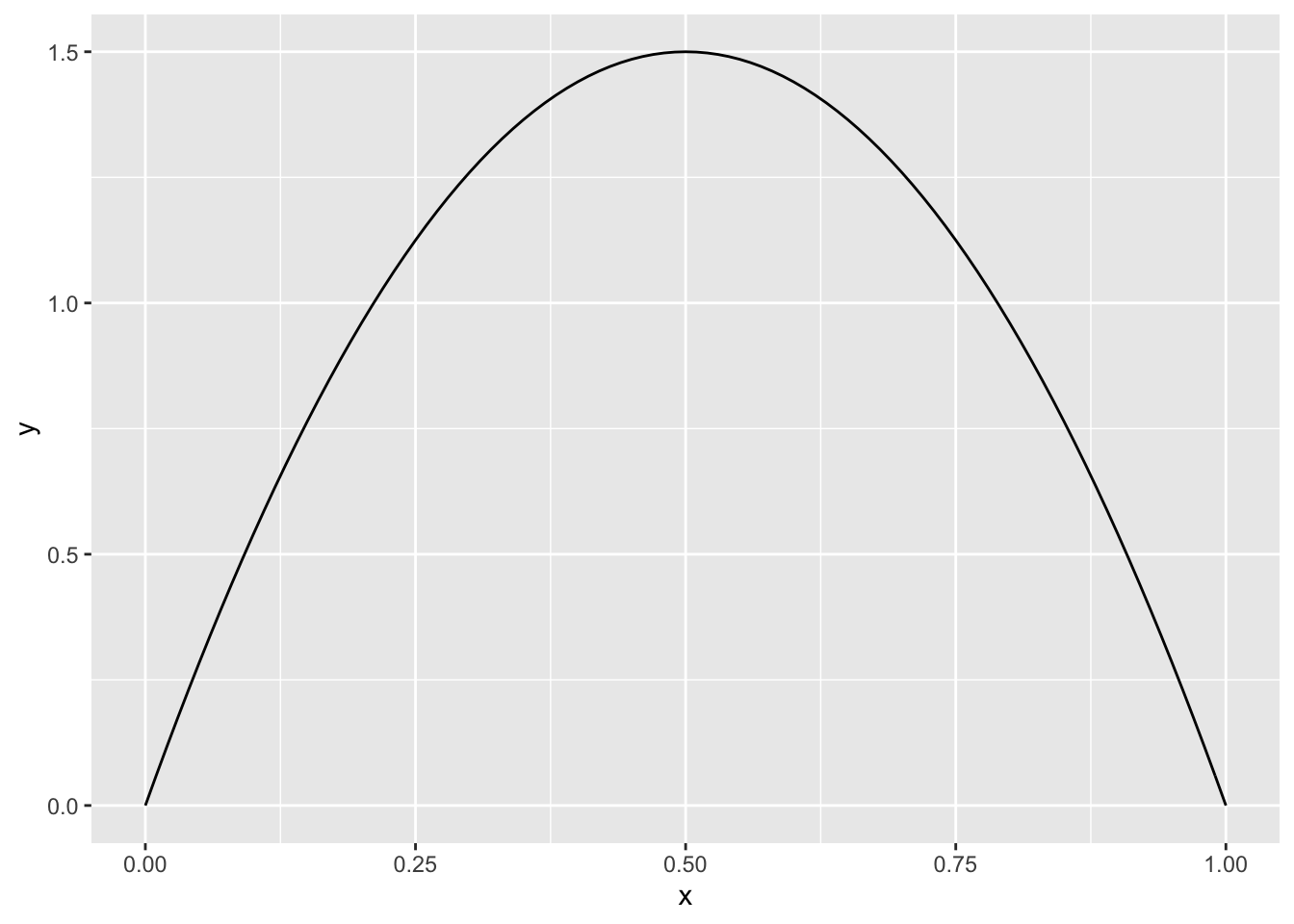
We start in the familiar one-dimensional case. Suppose we wish to take a random sample from a beta random variable with parameters \(\alpha = 2\) and \(\beta = 2\) without using rbeta. As a reminder, the pdf looks like this:
Now, we take a random sample of some large size from the possible outcomes of the rv \(X\) that we are sampling from. In this case, we take a random sample of size 50,000 on the interval \([0, 1]\).
These are the potential xs that we can get in our sample from \(X\). Note that this means that the number of potential samples should be considerably larger than the sample size that we are intending on taking. Next, we compute the likelihoods of each of the \(x\)-values, by evaluating the pdf at each \(x\).
Intuitavely, the probability of sampling something near an \(x\) is proportional to the pdf evaluated at that x. If the xs had been sampled on a uniform grid, then this would be exactly true. Then, we use sample to sample from the xs according to the probabilities in probs. Note that sample will automatically scale the probs so that they sum to 1, so we do not need to worry about that. THIS SHOULD BE THOUGHT THROUGH AND EXPLAINED BETTER
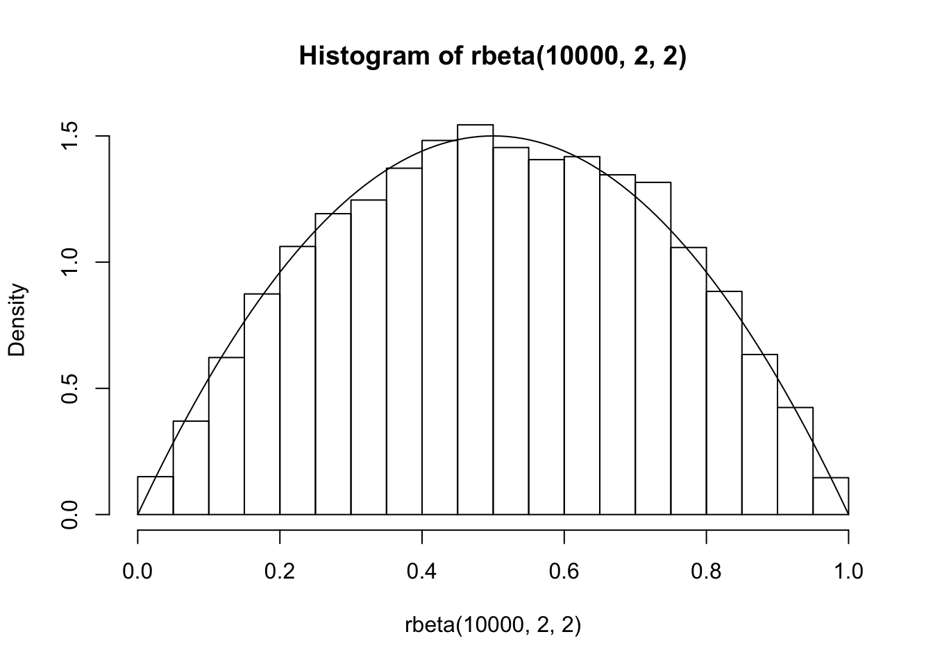
We can test to see whether this is working well by plotting a histogram and super-imposing the pdf of a beta(2,2) random variable.

We can also compare this to the match we would get if sampling using rbeta:
It is more challenging to apply this technique to random variables that are “peaky” or that have unbounded domain. Let’s see how to sample from a standard normal random variable. First, we decide that want a sample of size 10,000. We decide that with pretty good probability, all 10,000 samples will be within 4 standard deviations of the mean. So, we restrict to an interval \([-4, 4]\) to take our original random sample.
xs <- runif(50000, -4, 4)
probs <- dnorm(xs)
random_sample <- sample(xs, 10000, T, prob = probs)
hist(random_sample, probability = T)
curve(dnorm(x), add = T)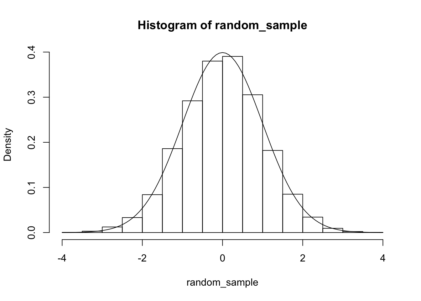
From this, we can see why a “peaky” distribution could cause problems for this technique. We need to allocate potential samples across all outcomes that fall within 4 standard deviations of the mean. However, by far the most outcomes will be within 2 standard deviations of the mean. So, we are allocating a lot of resources to unlikely regions, which limits the accuracy that we can get in the likely regions. In an extreme case, there may be only a very small region that is likely at all, and we may only have no potential samples that fall in that region! Nonetheless, for many common density functions, this technique works well to give an idea about what is going on, and is certainly good enough for understanding the relationship between sampling and theory. Finally, we point out that this technique will break down for high-dimensional data, as we would need too many points to get decent coverage of the plausible region. In Chapter 14, we will see an exact method for sampling from a one-dimensional distribution.
13.2.3 Two dimensional case
The two-dimensional case proceeds analogously to the one-dimensional case. We first find a bounded rectangle which most likely will contain all of the samples that we wish to take. We randomly select a large number of values from that rectangle as potential samples. Then, we sample from those points with probability proportional to the joint pdf evaluated at those points.
Consider the example presented above:
\[ f(x, y) = \begin{cases} x + y& 0\le x \le 1, 0 \le y \le 1 \\ 0& \mathrm{otherwise} \end{cases} \]
In this case, the rectangle that likely (definitely) contains all of the samples we wish to take is \([0, 1] \times [0,1]\). We store the potential samples in a data frame named dat, but we will also make use of xs and ys below.
xs <- runif(50000, 0, 1)
ys <- runif(50000, 0, 1)
dat <- matrix(c(xs, ys), ncol = 2)
dat <- data.frame(dat)
names(dat) <- c("x", "y")
Next, we define the joint pdf. This is a function of two variables, that we call x and y, and the formula for the pdf goes inside the function.
Finally, we sample from the indices of the data frame with probabilities proportional to the joint pdf evaluated at the corresponding \((x, y)\) coordinate inside the data frame.
Our sample is
We can visualize this via:
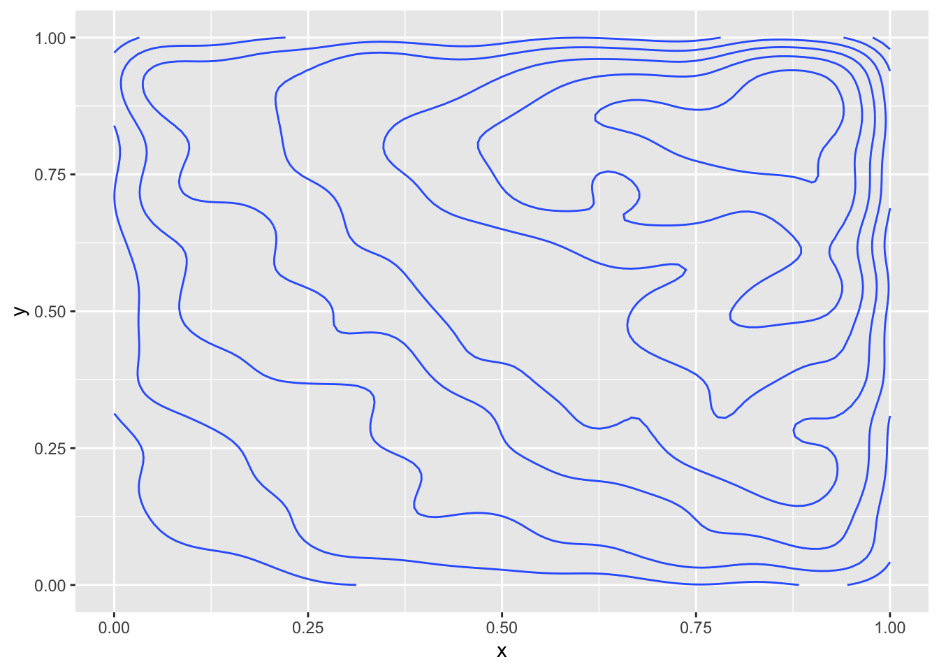
This gives the approximate level sets of the pdf. Note that the true level sets are when \(x + y = C\), so they should be lines with slope -1, which they approximately are. Some better visualizations are possible using the plotly package, which we will not discuss here.
Example Sample from a joing distribution given by \[ f(x, y) = \begin{cases} \text{dnorm(x) * dexp(y)} & y > 0\\ 0 & \text{otherwise} \end{cases} \]
A bounding rectangle in this case is approximately \([-4, 4] \times [0, 10]\). The following R code illustrates how to sample from this joint distribution.
N <- 500000
xs <- runif(N, -4, 4)
ys <- runif(N, 0, 10)
dat <- matrix(c(xs, ys), ncol = 2)
dat <- data.frame(dat)
names(dat) <- c("x", "y")
joint_pdf <- function(x, y) {
dnorm(x) * dexp(y)
}
probs <- joint_pdf(xs, ys)
indices <- sample(1:N, 10000, T, probs)
random_sample <- dat[indices,]
ggplot(random_sample, aes(x, y)) +
geom_density_2d()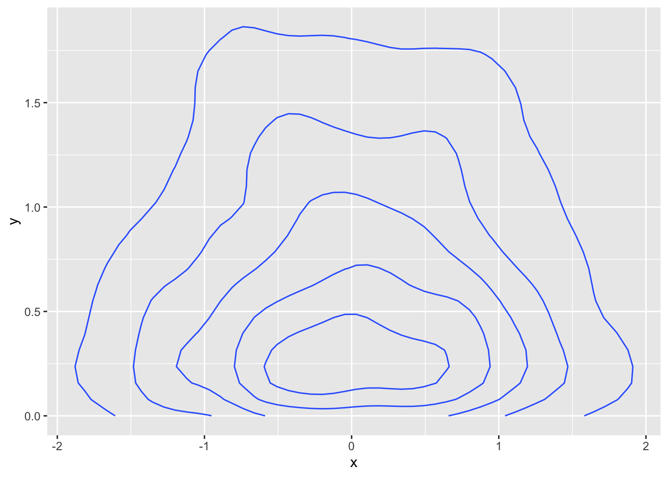
This indicates that the most likely value is close to \((0, 0)\) and that samples get generally less likely as we move away from that point, at differing speeds depending on the direction. One test we can do to see whether we need to take a denser sample inside of our original rectangle is to see how many of the samples are repeated. Ideally, we would like none of them to be repeated, but that is unlikely to occur.
## [1] 1024Here, we have about 10% of the total number of samples are duplicated, which for our purposes in this text will tend to lead to accurate estimations. An alternative way to increase the density in the rectangle is to decrease the rectangle size, which may lead to inaccurate estimates for rare events, but may be unavoidable in some situations. Again, we emphasize that our goal is a straightforward random sampling technique that will illustrate the ideas in the later sections; not the best possible technique.
Example Sampling from a joint pdf that doesn’t have a rectangular domain of definition.
Suppose we have joint pdf given by \[ f(x, y) = \begin{cases} 8 xy & 0\le y \le x \le 1\\0&\text{otherwise} \end{cases} \]
The only unique part of this is defining the joint pdf correctly.
N <- 200000
xs <- runif(N, 0, 1)
ys <- runif(N, 0, 1)
dat <- matrix(c(xs, ys), ncol = 2)
dat <- data.frame(dat)
names(dat) <- c("x", "y")
joint_pdf <- function(x, y) {
ifelse(y < x, 8 * x * y, 0) #use this because it is vectorized!
}
probs <- joint_pdf(xs, ys)
indices <- sample(1:N, 10000, T, probs)
sum(duplicated(indices)) #check less than 10%## [1] 839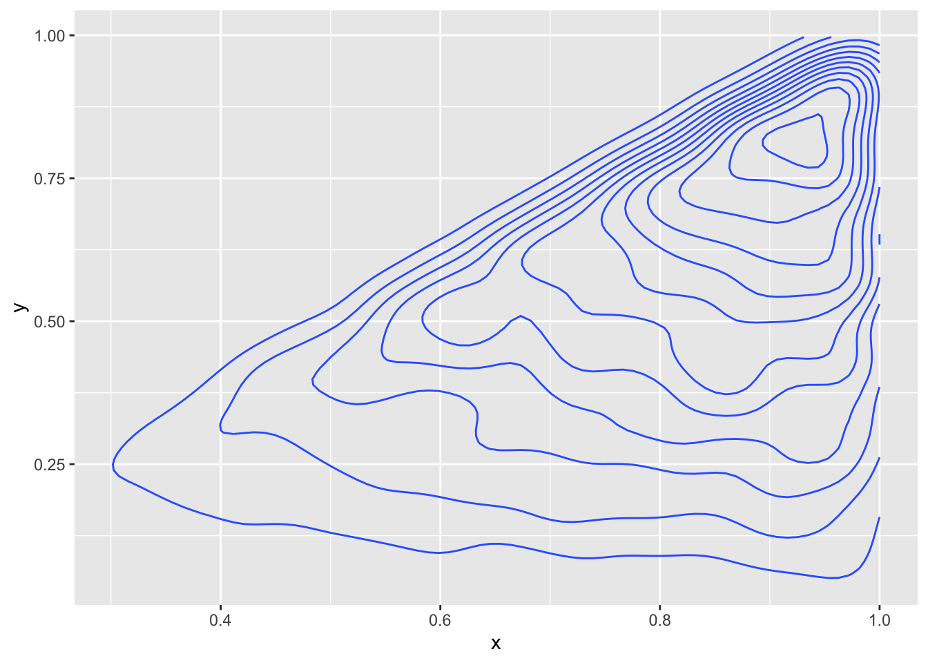
We will see a more efficient (and exact!) way to sample from the last two distributions later in this chapter.
13.3 Computing Probabilities and Expectations
In this short section, we see how to compute probabilities and expected values given a joint pdf.
Example Let \(X\), \(Y\) be random variables with joint density given by
\[ f(x, y) = \begin{cases} x + y & 0 \le x, y\le 1 \\ 0 &\text{otherwise}\end{cases} \]
Find \(P(X > 1/2)\). To do this, we integrate the joint density over the region defined by \(x > 1/2\). Namely, \[ \begin{aligned} \int_0^1 \int_{1/2}^1 x + y\, dx dy &= \int_0^1 1/2 x^2 + xy|_{x = 1/2}^1 \\ &= \int_0^1 3/8 + 1/2 y \, dy\\ &= 3/8 y + 1/4 y^2|_{y = 0}^1 = 3/8 + 1/4 = 5/8 \end{aligned} \]
Find \(P(Y < X)\). Again, we need to integrate over the region defined by \(y < x\). Namely, \[ \begin{aligned} \int_0^1 \int_{0}^x x + y\, dy dx &= \int_0^1 1/2 y^2 + xy|_{y = 0}^x \\ &= \int_0^1 3/2 x^2 \, dx\\ &= 1/2 \end{aligned} \]
Example Estimate the probabilities above using random sampling.
We begin by getting a random sample from the joint distribution of \(X\) and \(Y\), as in the previous section.
xs <- runif(50000, 0, 1)
ys <- runif(50000, 0, 1)
dat <- matrix(c(xs, ys), ncol = 2)
dat <- data.frame(dat)
names(dat) <- c("x", "y")
joint_pdf <- function(x, y) {
  x + y
}
probs <- joint_pdf(xs, ys)
indices <- sample(1:50000, 10000, T, probs)
sum(duplicated(indices)) #around 10%## [1] 1077Now, we simply find the proportion of times that \(X > 1/2\) and that \(Y < X\).
The following is an estimate for \(P(X > 1/2)\).
## [1] 0.6362And to estimate \(P(Y < X)\),
## [1] 0.5066Given a joint pdf \(f\) of \(X\) and \(Y\) and a function \(g(x, y)\), we can compute \[ E[g(X, Y)] = \int \int g(x, y) f(x, y)\, dx dy. \] The bounds of integration are ostensibly from \(-\infty\) to \(\infty\), but we reduce down to where the pdf is positive and only integrate over that region.
Example Let \(f\) be the joint density function given above. Compute the following expected values.
- \(E[X] = \int_0^1 \int_0^1 x (x + y) \, dx dy = 7/12\)
- \(E[XY] = \int_0^1 \int_0^1 xy(x + y)\, dxdy = 1/3\)
- \(E[X^2] = \int_0^1 \int_0^1 x^2 (x + y)\, dxdy = 5/12\)
Recall that the covariance of \(X\) and \(Y\) is \[ E[(X - \mu_X) (Y - \mu_Y)] = E[XY] - E[X]E[Y], \] We expect to see a positive covariance if increased values of \(X\) are probabilistically associated with increased values of \(Y\), and we expect to see a negatice covariance when increased values of \(X\) are associated with decreased values of \(Y\). In the example under consideration, it is not immediately clear from the joint density whether we expect a positive or a negative covariance, but see below for examples where it is more clear.
In our example under consideration, the covariance is \(1/3 - (7/12)^2 = -.006944\). Finally, we often scale the covariance by dividing by the standard deviations of \(X\) and \(Y\) to get the correlation.
Recall also that the correlation of \(X\) and \(Y\) is given by \[ \rho(X, Y) = \frac{E[(X - \mu_X) (Y - \mu_Y)]}{\sigma_X \sigma_Y} \]
In the example under consideration, we compute \(\sigma_X = \sqrt{E[X^2] - \mu_X^2} = \sqrt{5/12 - (7/12)^2} = .276\). Therefore, the correlation of \(X\) and \(Y\) is \[ \frac{E[XY] - E[X]E[Y]}{\sigma_X \sigma_Y} = -.006944/(.2763854)^2 = -.09 \]
The correlation is often more useful than the covariance, since correlation varies from \(-1\) to \(1\), with the extremes corresponding to a perfect linear relationship between \(X\) and \(Y\). In the case under consideration, the correlation is relatively close to zero, so the variables are weakly negatively correlated.
Theorem 3.10 Let \(X\) and \(Y\) be random variables and let \(a\) and \(b\) be constants. \[ V(aX + bY) = a^2 V(X) + b^2V(Y) + 2ab {\text{Cov}}(X, y) \]
Proof. From the definition of variance, we have that \(V(aX + bY) = E[(aX + bY)^2] - E[aX + bY]^2\). We compute the two quantities separetely and do some algebra to get the result.
\[ \begin{aligned} E[(aX + bY)^2] &= E[a^2X^2 + ab XY + b^2 Y^2]\\ &=a^2E[X^2] + abE[XY] + b^2 E[Y^2] \end{aligned} \]
while \[ \begin{aligned} E[aX + bY]^2 &= a^2E[X]^2 + 2ab E[X]E[Y] + b^2 E[Y]^2. \end{aligned} \]
Therefore, \[ \begin{aligned} V(aX + bY) &= a^2(E[X^2] - E[X]^2) + b^2(E[Y^2] - E[Y]^2) + 2ab (E[XY] - E[X]E[Y])\\ &= a^2V(X) + b^2 V(Y) + 2ab {\text{Cov}}(X, Y), \end{aligned} \] as desired.
In particular, we have proven the following theorem in the case that there are only two random variables in question
(#thm:variance_independent) If \(X_1, \ldots, X_n\) independent then \(V(\sum_{i=1}^n a_i X_i) = \sum_{i = 1}^n a_i^2 V(X_i)\).
We end this section by estimating all of the above quantities using our random sample from the joint density. We simply take the average value from our sample of the quantity indicated in order to estimate the expected value.
## [1] 0.5890656## [1] 0.3356352## [1] 0.4229929To estimate the covariance and correlation, we can use the built in R functions cov and cor.
## [1] -0.006115894## [1] -0.0797139913.4 Marginal and Conditional Densities
Given a joint density for \(X\) and \(Y\), we define the marginal density of \(X\) to be \[ f_X(x) = \int_{-\infty}^\infty f(x, y)\, dy \] and the marginal density of \(Y\) to be \[ f_Y(y) = \int_{-\infty}^\infty f(x, y)\, dx \] As usual, we restrict the integral to the region where \(f\) is positive when that is not the entire plane.
Example Consider \[ f(x, y) = \begin{cases} x + y& 0\le x \le 1, 0 \le y \le 1 \\ 0& \mathrm{otherwise} \end{cases} \] The marginal density of \(X\) is given by \[ \begin{aligned} f_X(x) &= \int_{-\infty}^\infty f(x, y)\, dy \\ &=\int_{0}^1 x + y \, dy\\ &= x + 1/2 \end{aligned} \]
For \[ f(x, y) = \begin{cases} 8 xy & 0\le y \le x \le 1\\0&\text{otherwise} \end{cases} \] we have \[ \begin{aligned} f_Y(y) &= \int_{-\infty}^\infty f(x, y)\, dx\\ &= \int_{y}^1 8xy\, dx\\ &=4x^2y|_{x = y}^1\\ &=4y - 4y^3 \end{aligned} \]
For \[ f(x, y) = \begin{cases} \text{dnorm(x) * dexp(y)} & y > 0\\ 0 & \text{otherwise} \end{cases} \] we have that integrating out \(X\) yields 1 for every \(y\), so \(f_Y(y) = \text{dexp(y)}\).
Let’s confirm these calculations from our sampling procedures. Once we have a sample from the joint density function, we can simply ignore the variable we are not interested in, and that is a sample from the marginal density of the variable we are interested in!
For the first problem above:
xs <- runif(50000, 0, 1)
ys <- runif(50000, 0, 1)
dat <- matrix(c(xs, ys), ncol = 2)
dat <- data.frame(dat)
names(dat) <- c("x", "y")

joint_pdf <- function(x, y) {
  x + y
}
probs <- joint_pdf(xs, ys)

indices <- sample(1:50000, 10000, T, probs)
sum(duplicated(indices)) #around 10%
## [1] 1109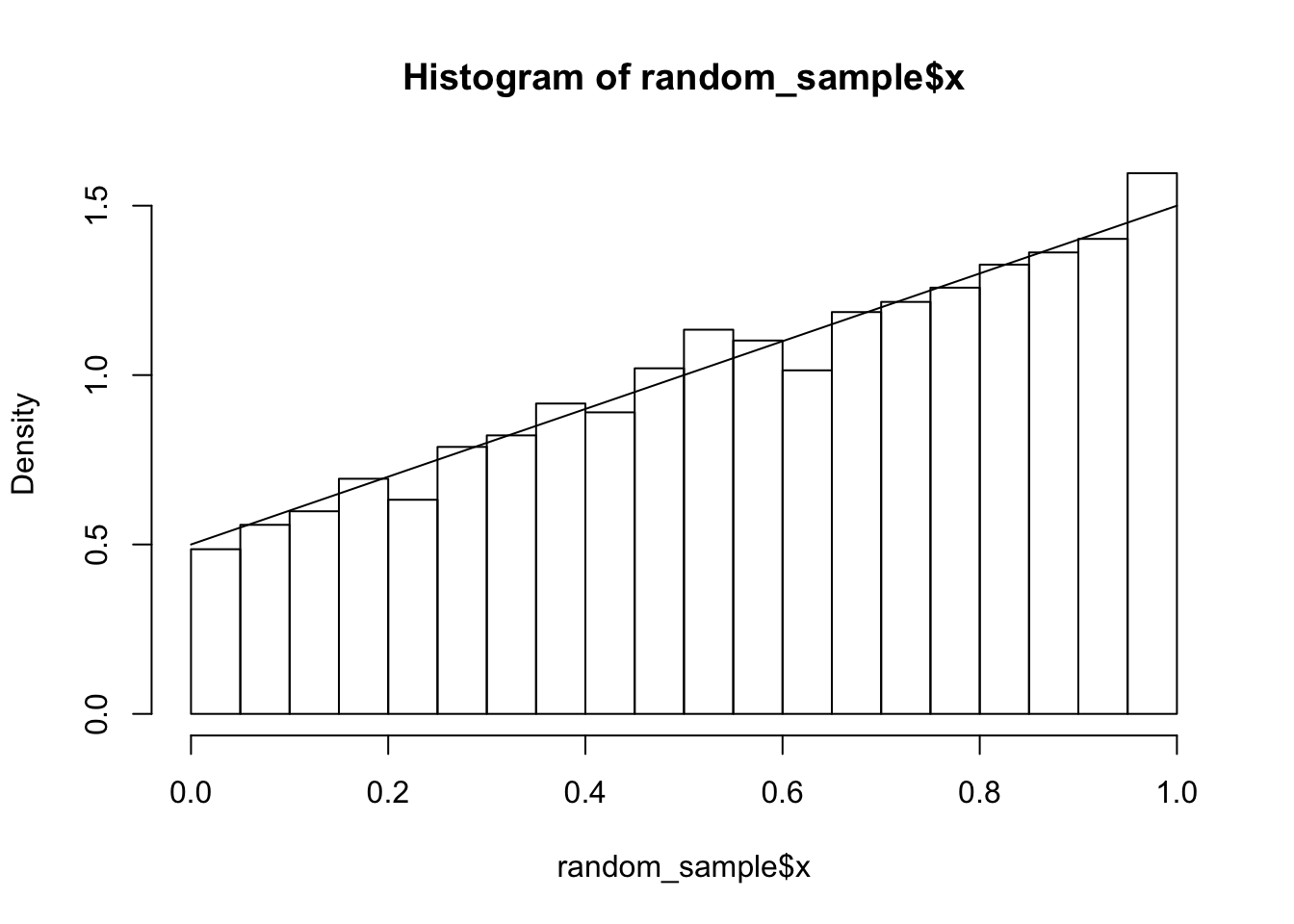
We see that we have a pretty good match to the histogram, which confirms our computations above.
For the second example:
N <- 200000
xs <- runif(N, 0, 1)
ys <- runif(N, 0, 1)
dat <- matrix(c(xs, ys), ncol = 2)
dat <- data.frame(dat)
names(dat) <- c("x", "y")

joint_pdf <- function(x, y) {
  ifelse(y < x, 8 * x * y, 0)
}
probs <- joint_pdf(xs, ys)

indices <- sample(1:N, 10000, T, probs)
random_sample <- dat[indices,]
hist(random_sample$y, probability = T)
curve(4*x - 4*x^3, add = T)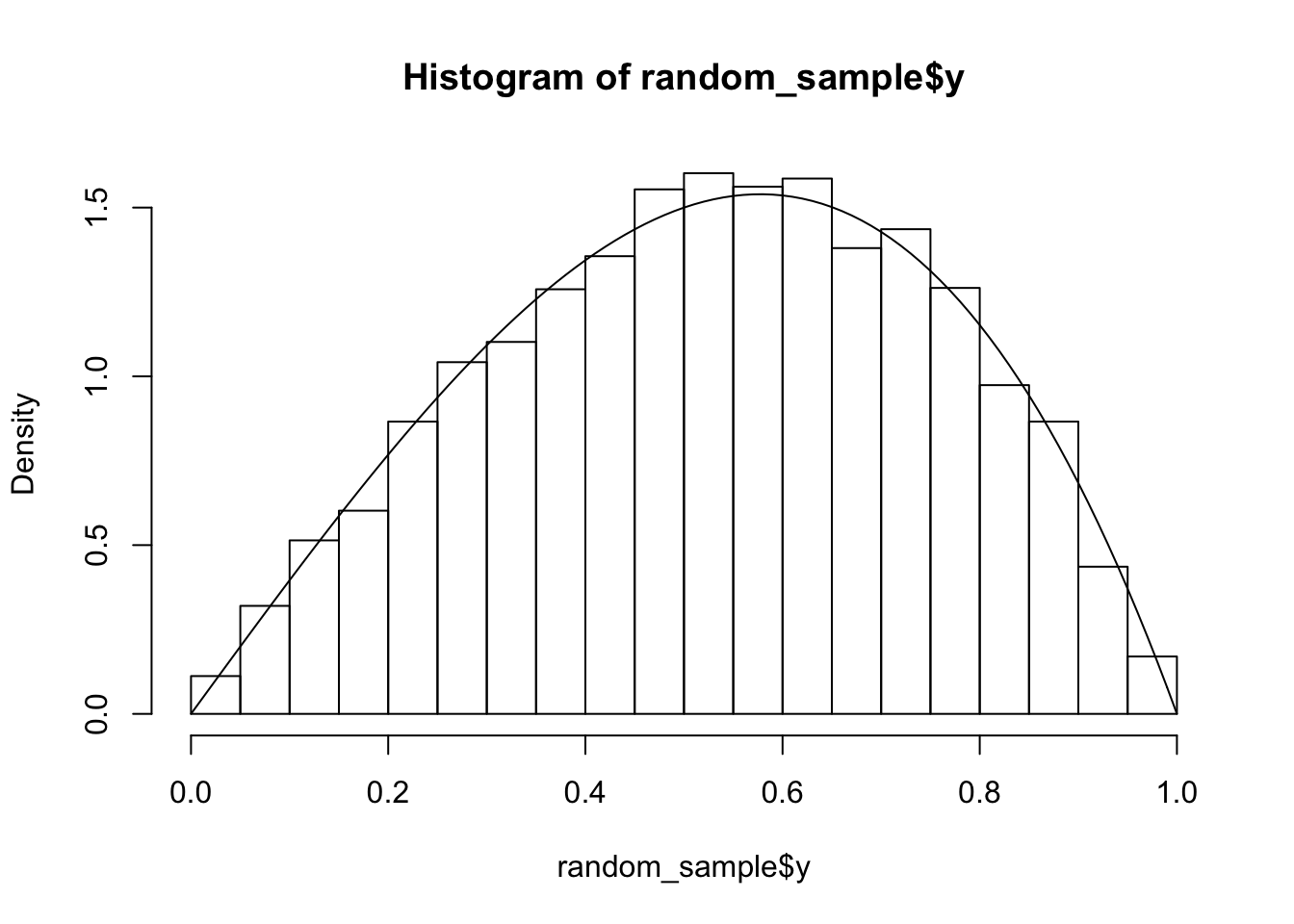
Again, we see that the simulations match the theoretical computation.
The **conditional density* of \(X\) given \(Y = y\) is defined by \[ f(X|Y = y) = \frac{f(x, y)}{f_Y(y)} \] By symmetry, \[ f(Y|X = x) = \frac{f(x, y)}{f_X(x)} \]
Since we have already computed the marginals above, it is simple to compute the conditional densities.
For \[ f(x, y) = \begin{cases} x + y& 0\le x \le 1, 0 \le y \le 1 \\ 0& \mathrm{otherwise} \end{cases} \] we have \(f(X|Y = 1/3) = f(x, 1/3)/f_Y(1/3) = (x + 1/3)/(1/3 + 1/2) = 6/5 x + 2/5\), \(0\le x \le 1\). It is easy to simulate values from this conditional density: we simply set \(y = 1/3\) in the joint pdf and do one-dimensional sampling.
joint_pdf <- function(x, y) {
  x + y
}

xs <- runif(50000, 0, 1)
probs <- joint_pdf(xs, 1/3)

random_sample <- sample(xs, 10000, T , prob = probs)
hist(random_sample, probability = T)
curve(6/5 * x + 2/5, add = T)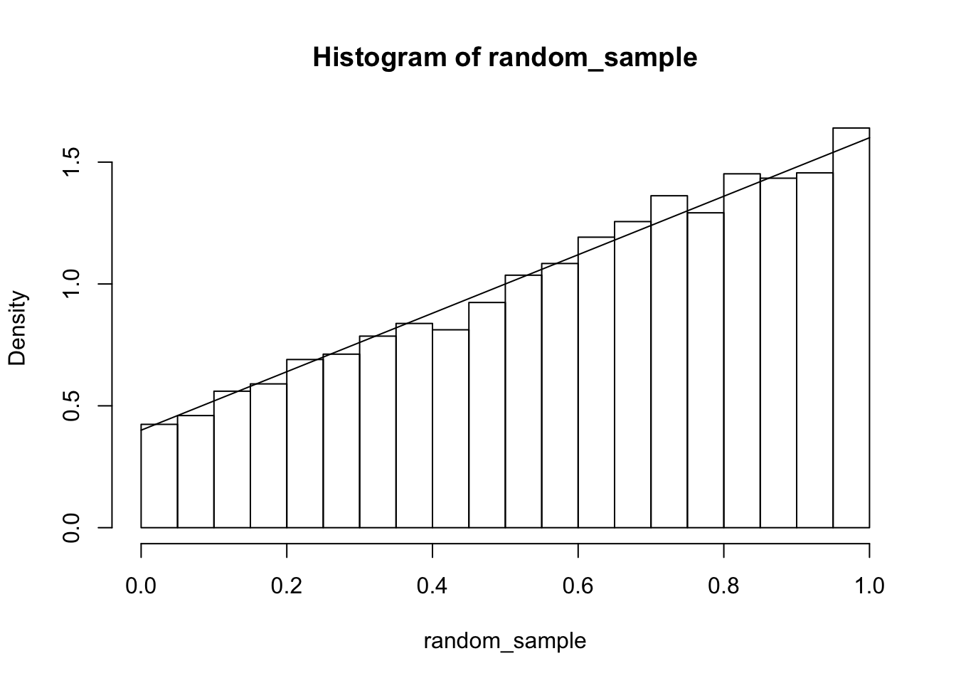
When the region where \(f\) is positive is not a rectangle, we need to be careful to keep track of which values are possible in the conditional density. For example, if \[ f(x, y) = \begin{cases} 8 xy & 0\le y \le x \le 1\\0&\text{otherwise} \end{cases} \] then \(f(X|Y = 1/2) = 4x/f_Y(1/2)\) when \(1/2 \le x \le 1\). Note the region for which this is valid!! Noting that \(f_Y(1/2) = 3/2\), we get \(f(X|Y = 1/2) = 8/3 x\), \(1/2 \le x \le 1\). Let’s verify via simulation.
joint_pdf <- function(x, y) {
  ifelse(y < x, 8 * x * y, 0)
}
xs <- runif(100000, 0, 1) #better would be to restrict to possible values!
probs <- joint_pdf(xs, 1/2)

random_sample <- sample(xs, 10000, T , prob = probs)
hist(random_sample, probability = T)
curve(8/3 * x, add = T)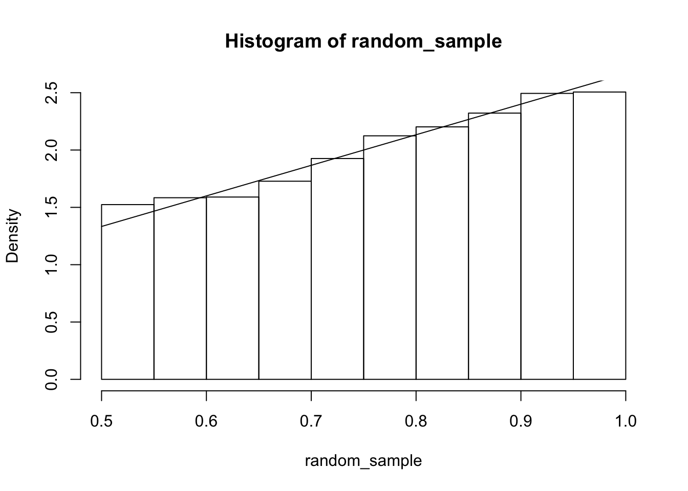
13.5 Independence
We previously defined independence of random variables \(X\) and \(Y\) by \(P(X \le x, Y \le y) = P(X \le x) P(Y \le y)\) for all \(x, y\). In terms of pdfs, this means that the joint pdf of \(X\) and \(Y\) factors into the product of a function just in terms of \(x\) and a function that is just in terms of \(y\). In particular, if \(R\) is the region of the plane for which \(f(x, y) > 0\), then in order for \(X\) and \(Y\) to be independent, it must be true that \(R = A \times B\) for some sets \(A\) and \(B\).
Example For the three joint distributions that we defined above, \[ f(x, y) = \begin{cases} x + y& 0\le x \le 1, 0 \le y \le 1 \\ 0& \mathrm{otherwise} \end{cases} \] yields dependent random variables, because there is no way to write \(x + y\) as a function of \(x\) times a function of \(y\).
The joint pdf
\[
f(x, y) = \begin{cases} 8 xy & 0\le y \le x \le 1\\0&\text{otherwise} \end{cases}
\]
also describes dependent random variables, because the region over which the random variable is positive cannot be written as \(A \times B\).
The joint pdf
\[
f(x, y) = \begin{cases}
\text{dnorm(x) * dexp(y)} & y > 0\\
0 & \text{otherwise}
\end{cases}
\]
describes independent random variables, because the region over which the random variables are positive is \((-\infty, \infty) \times [0, \infty)\) and the function factors as dnorm(x) times dexp(y).
In the case that the random variables \(X\) and \(Y\) are independent, it follows that in fact, \(f(x, y) = f_X(x) f_Y(y)\). This fact is useful for proving some facts about expectations.
Theorem: If \(X\) and \(Y\) are independent and \(g(X, Y) = h(X) k(Y)\), then \(E[g(X, Y)] = E[h(X)]E[k(Y)]\)
Proof: \[ \begin{aligned} E[g(X, Y)] &= \int \int h(X) k(Y) f_X(x) f_Y(y)\, dxdy \\ &= \int h(X) f_X(x)\, dx \int k(Y) f_Y(y)\, dy\\ &= E[h(X)]E[k(Y)] \end{aligned} \]
In particular, \(E[XY] = E[X]E[Y]\), so independence implies correlation equals zero. Note that the converse is not true. It is possible to have uncorrelated random variables that are not independent. The simplest example may be the following. Let \(X\) be a standard normal random variable, and \(Y = X^2\). Clearly, \(X\) and \(Y\) are far from independent, because knowing \(X\) tells me exactly what \(Y\) is! However, \(E[XY] = E[X^3] = \int x^3 dnorm(x)\, dx = 0\), since \(x^3 dnorm(x)\) is an odd function. Additionally, \(E[X] = 0\), so \(E[XY] - E[X]E[Y] = 0\), and \(X\) and \(Y\) are uncorrelated.