Chapter 11 Analysis of Variance and Comparison of Multiple Groups

In this chapter, we introduce one-way analysis of variance (ANOVA) through the analysis of a motivating example. In a study of the effects of marijuana on mice, wild type mice were given either a vehicle or a dose of marijuana based on their body weight. Various measurements were performed, one of which was a measurement of the percent of baseline locomotion in the mice. For more information, see this paper ³⁷

The data is in the fosdata package in the mice_pot data set .

mice_pot <- fosdata::mice_pot

The data consists of 42 observations of 2 variables. The variable group is the dosage of THC that the mouse received, and percent_of_act is the percent of baseline locomotion. The vehicle denotes a control-type measurement, where the mouse was given a shot with the same inactive ingredients but no THC. Let’s look at some summary data and plots.

mice_pot %>% 
  group_by(group) %>% 
  summarize(mean = mean(percent_of_act),
            sd = sd(percent_of_act), 
            skew = e1071::skewness(percent_of_act),
            N = n()) %>% 
  knitr::kable(digits = 3)

## `summarise()` ungrouping output (override with `.groups` argument)

group	mean	sd	skew	N
VEH	100.000	25.324	-0.190	15
0.3	97.323	31.457	0.133	9
1	99.052	26.258	-0.106	12
3	70.668	20.723	0.034	10

Now let’s look at a boxplot.

ggplot(mice_pot, aes(x = group, y = percent_of_act)) +
  geom_boxplot(outlier.size = -1) +
  geom_jitter(height = 0, width = .2)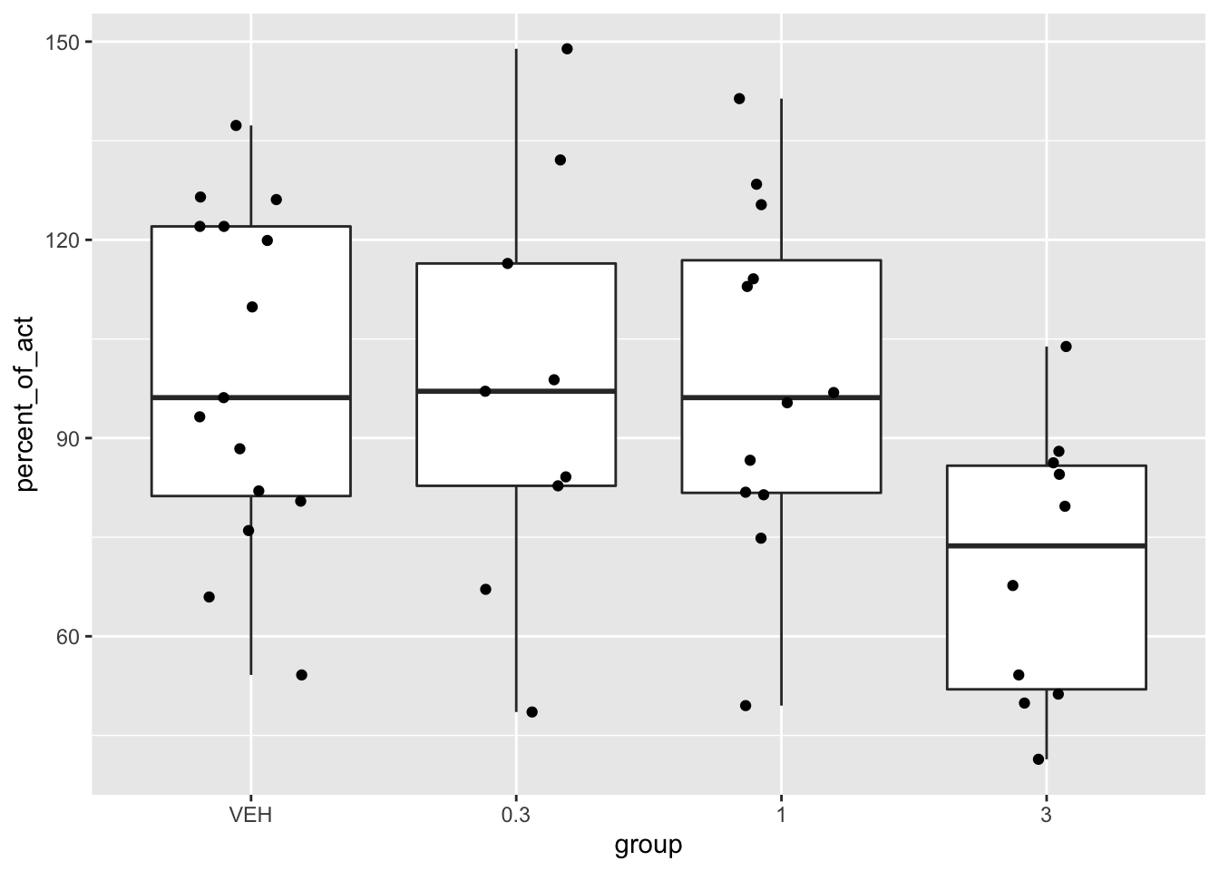

Looking at the plot and the summary statistics, it seems unlikely that there is any difference in the first three groups, but there may well be a difference once the dose gets up to 3 mg/kg. Another thing to notice is that the data is not very skew, and it is at least plausibly approximately normal. ANOVA is a method for testing whether the mean percent of activity relative to baseline is the same in all four groups, under the assumption of normality of each group, independence and equal variance.

In this chapter, we will discuss ANOVA in detail, and we will also briefly discuss oneway.test.

11.1 Setup

Notation

$x_{ij}$ denotes the $j$th observation from the $i$th group.
$\overline{x}_{i\cdot}$ denotes the mean of the observations in the $i$th group.
$\overline{x}_{\cdot}$ denotes the mean of all observations.
There are $k$ groups.
There are $n_i$ observations in the $i$th group.
There are $N$ total observations.

As an example, in mice_pot, there are 4 groups. We have $x_{11} = 54.2, x_{12} = 65.9, \ldots, x_{21} = 98.8,\ldots,x_{31} = 95.3,\ldots$ and so on. This is because, looking at the data frame arranged by group, the first percent activity is $54.2$, and associated with VEH. The second percentage of activity associated with VEH is $65.9$. The first temperature difference associated with 0.3 mg/kg is $98.8$.

To compute the group means:

mice_pot %>% 
  group_by(group) %>% 
  summarize(round(mean(percent_of_act), 1))

## `summarise()` ungrouping output (override with `.groups` argument)

## # A tibble: 4 x 2
##   group `round(mean(percent_of_act), 1)`
##   <fct>                            <dbl>
## 1 VEH                              100  
## 2 0.3                               97.3
## 3 1                                 99.1
## 4 3                                 70.7

This tells us that $\overline{x}_{1\cdot} = 100$, for example. This is because the percentage of activity has been normalized to the vehicle group, so that 100 percent is by definition what the vehicle group did.

To get the overall mean, we use mean(cows$temp_diff), which is $92.9$.

Our model for the percentage of activity is \[ x_{ij} = \mu + \alpha_i + \epsilon_{ij}, \] where $\mu$ is the grand mean, $\alpha_i$ represents the difference between the grand mean and the group mean, and $\epsilon_{ij}$ represents the variation within the group. So, each individual data point could be realized as \[ x_{ij} = \overline{x}_\cdot + (\overline{x}_{i\cdot} - \overline{x}) + (x_{ij} - \overline{x}_{i\cdot}) \]

The null hypothesis for ANOVA is that the group means are all equal (or equivalently all of the $\alpha_i$ are zero). So, if $\mu_i = \mu + \alpha_i$ is the true group mean, we have:

\[ H_0 : \mu_1 = \mu_2 = \cdots =\mu_k\\ H_a : \text{Not all $\mu_i$ are equal} \]

11.2 ANOVA

ANOVA is “analysis of variance” because we will compare the variation of data within individual groups with the overall variation of the data. We make assumptions (below) to predict the behavior of this comparison when $H_0$ is true. If the observed behavior is unlikely, it gives evidence against the null hypothesis. The general idea of comparing variance within groups to the variance between groups is applicable in a wide variety of situations.

Define the variation within groups to be \[ SSD_W = \sum_i \sum_j (x_{ij} - \overline{x}_{i\cdot})^2 \] and the variation between groups to be \[ SSD_B = \sum_i\sum_j (\overline{x}_{i\cdot} - \overline{x})^2 \] and the total variation to be \[ SSD_{tot} = \sum_i \sum_j (\overline{x} - x_{ij})^2. \]

Theorem 7.2 With the above notation, $SSD_{tot} = SSD_W + SSD_B$.

This says that the total variation can be broken down into the variation between groups plus the variation within the groups. If the variation between groups is much larger than the variation within groups, then that is evidence that there is a difference in the means of the groups. The question then becomes: how large is large? In order to answer that, we will need to examine the $SSD_B$ and $SSD_W$ terms more carefully. At this point, we also will need to make

Assumptions

The population is normally distributed within each group
The variances of the groups are equal. (Yikes!)
The observations are independent. One common way that this fails for one-way ANOVA is by using the same unit in each group. In the mice example, if each mouse had been given the vehicle and the 3 dosings of THC, then we would not be able to assume independence, and a different technique would be needed.

Recall: We have $k$ groups. There are $n_i$ observations in group $i$, and $N = \sum n_i$ total observations.

Notice that $SSD_W$ is almost $\sum\sum (\overline{x}_{ij} - \mu_i)^2$, in which case $SSD_W/\sigma^2$ would be a $\chi^2$ random variable with $N$ degrees of freedom. However, we are making $k$ replacements of means by their estimates, so we subtract $k$ to get that $SSD_B/\sigma^2$ is $\chi^2$ with $N - k$ degrees of freedom. (This follows the heuristic we started in Section 9.4).

As for $SSD_B$, it is trickier to see, but $\sum_i \sum_j (x_{i\cdot} - \mu)^2/\sigma^2$ would be $\chi^2$ with $k$ degrees of freedom. Replacing $\mu$ by $\overline{x}$ makes $SSD_B/\sigma^2$ a $\chi^2$ rv with $k - 1$ degrees of freedom.

The test statistic for ANOVA is: \[ F = \frac{SSD_B/(\sigma^2(k - 1))}{SSD_W/(\sigma^2(N - k))} = \frac{SSD_B/(k - 1)}{SSD_W/(N - k)} \]

This is the ratio of two $\chi^2$ rvs divided by their degrees of freedom; hence, it is $F$ with $k - 1$ and $N - k$ degrees of freedom. Through this admittedly very heuristic derivation, you can see why we must assume that we have equal variances (otherwise we wouldn’t be able to cancel the unknown $\sigma^2$) and normality (so that we get a known distribution for the test statistic).
If $F$ is much bigger than 1, then we reject $H_0: \mu_1 = \mu_2 = \cdots =\mu_k$ in favor of the alternative hypothesis that not all of the $\mu_i$ are equal.

We can also run simulations to see that the test statistic under the null hypothesis has an F distribution. Let’s assume that we have three populations, all of which are normally distributed with mean 0 and standard deviation 1 (recall that we must assume equal variances, and we are simulating the distribution of the test statistic under the null hypothesis, that all means are equal). We assume that we have 10 samples from group 1, 20 from group 2 and 30 from group 3. In the notation above, $k = 3$ and $N = 60$.

three_groups <- data.frame(group = rep(1:3, times = c(10, 20, 30)),
                           value = rnorm(60, 0, 1))

We could use built in R functions (as below) to compute the test statistic, but it is worthwhile to make sure we understand all of the formulas so we do it by hand. We first make sure that group is a factor! We can also check that (in this case, anyway) $SSE_W + SSE_B = SSE_{tot}$.

three_groups$group <- factor(three_groups$group)
sse <- three_groups %>% 
  mutate(total_mean = mean(value)) %>% 
  group_by(group) %>% 
  mutate(mu = mean(value), 
         diff_within = value - mu, 
         diff_between = mu - total_mean,
         diff_tot = value - total_mean) %>% 
  ungroup() %>% 
  summarize(sse_within = sum(diff_within^2),
            sse_between = sum(diff_between^2),
            sse_total = sum(diff_tot^2)) 
sse

## # A tibble: 1 x 3
##   sse_within sse_between sse_total
##        <dbl>       <dbl>     <dbl>
## 1       62.5        3.50      66.0

Now that we have computed the three sums of squared errors, we verify that $SSE_W + SSE_B = SSE_{tot}$.

sse$sse_within + sse$sse_between - sse$sse_total

## [1] 0

Now we can compute the test statistic.

k <- 3
N <- 60
(sse$sse_between/(k - 1))/(sse$sse_within/(N - k))

## [1] 1.59773

The R command for computing this directly, which we will use inside of our simulation since it is faster, is given by

aov.mod <- anova(lm(value ~ group, data = three_groups))
aov.mod$`F value`[1]

## [1] 1.59773

Now we are ready for our simulation.

sim_data <- replicate(1000, {
  three_groups <- data.frame(group = rep(1:3, times = c(10, 20, 30)),
                           value = rnorm(60, 0, 1))
  three_groups$group <- factor(three_groups$group)
  aov.mod <- anova(lm(value ~ group, data = three_groups))
  aov.mod$`F value`[1]
})
plot(density(sim_data),
     main = "F test statistic")
curve(df(x, 2, 57), add = T, col = 2)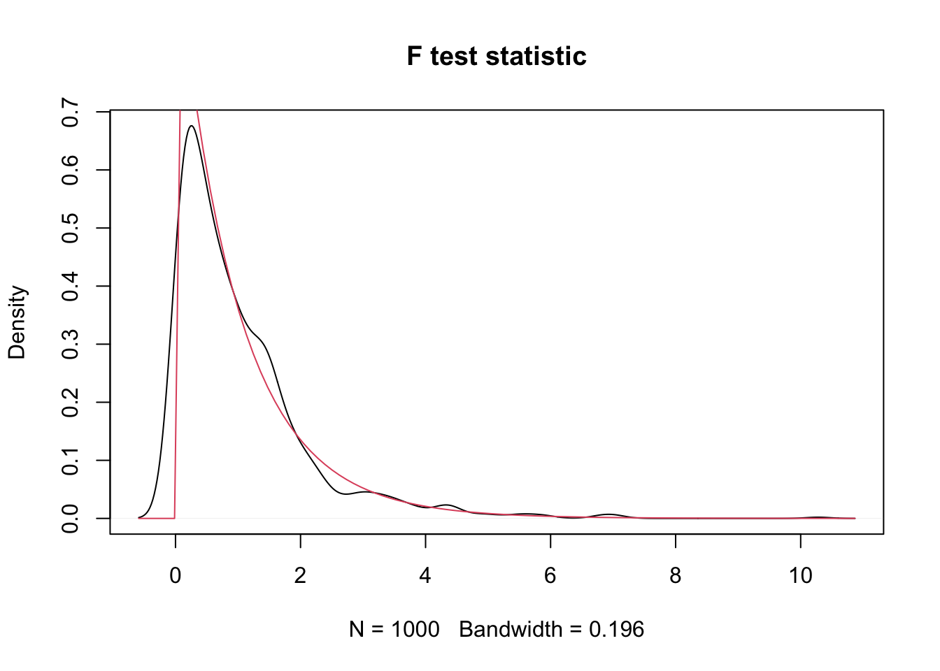

We see that, indeed, the test statistic looks approximately $F$ with 2 and 57 degrees of freedom.

11.3 Examples

11.3.1 Humanization

This paper studies the effect that learning about another group’s generosity can have on ones opinions about the other group. Participants were read a brief synopsis of Hurricane Katrina, and then either

told nothing further (control)
Told about the aid that Pakistan sent, but given low numbers for the amount aid.
Told about the aid that Pakistan sent, but given high numbers for the amount of aid.

Afterwards, the participants were asked how strongly they believed Pakistanis would have felt both secondary and primary emotions following the disaster, and the mean of their responses was taken.

We plan on analyzing whether there is a difference in the mean of the three groups’ belief of how strongly Pakistani’s would have felt secondary emotions. You can read more about the experiment in the help page for the data, or by reading the linked paper. One issue with the technique that we are using is that we are averaging the ordinal scale responses to the seven questions on emotions, which is a common, but not always valid, thing to do.

We can load the data via the following.

humanization <- fosdata::humanization

We will first examine the data to see whether it appears to be approximately normal with equal variances across the groups. We are only concerned in this problem with the people who were told about Hurricane Katrina.

kat_humanization <- humanization %>% filter(stringr::str_detect(group, "Kat"))
ggplot(kat_humanization, aes(x = group, y = pak_sec)) +
  geom_boxplot() +
  geom_jitter(height = 0, width = 0.2)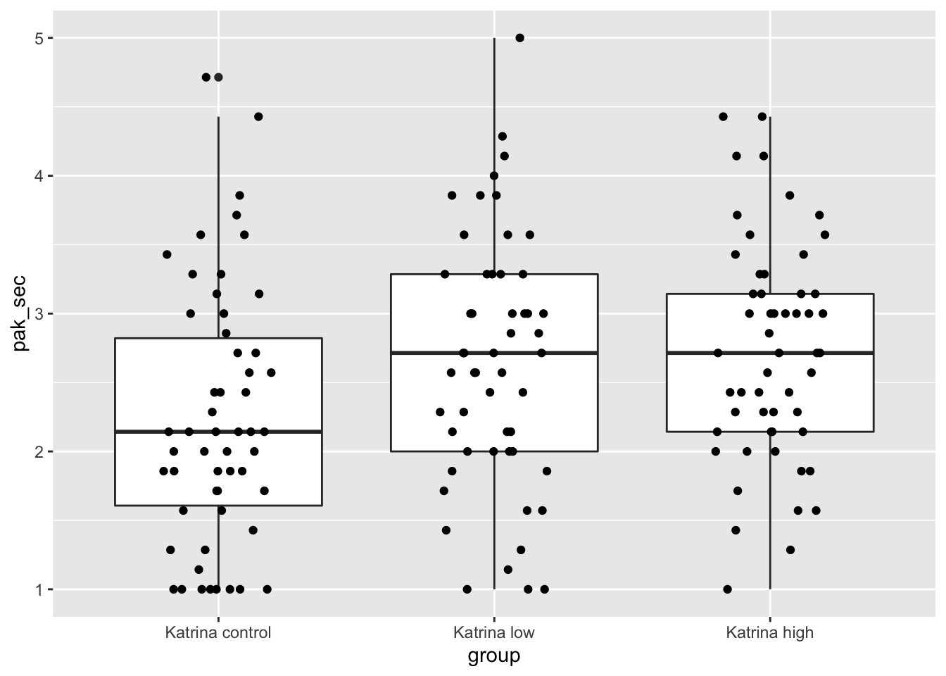

Those don’t look too bad, except that the control group and the low group both have more values exactly equal to 1 than would be expected in a normal distribution. Let’s look at the mean, standard deviation and sample size in each group.

kat_humanization %>% 
  group_by(group) %>% 
  summarize(mean = mean(pak_sec),
            sd = sd(pak_sec),
            n = n())

## `summarise()` ungrouping output (override with `.groups` argument)

## # A tibble: 3 x 4
##   group            mean    sd     n
##   <fct>           <dbl> <dbl> <int>
## 1 Katrina control  2.24 0.927    54
## 2 Katrina low      2.65 0.911    53
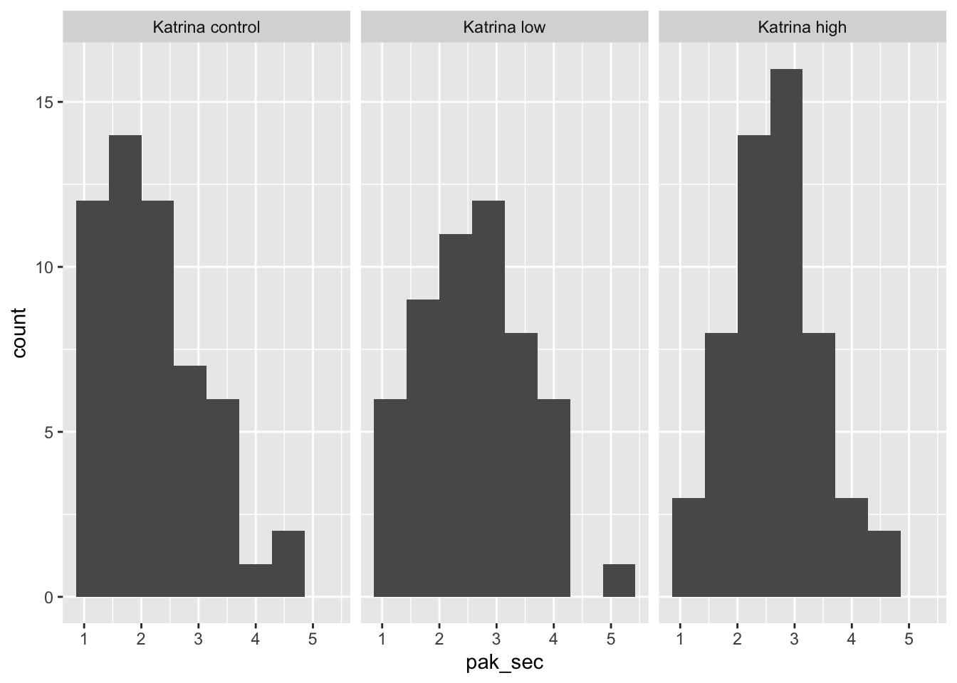
## 3 Katrina high     2.72 0.794    54

It’s probably also a good idea to do a histogram.

ggplot(kat_humanization, aes(x = pak_sec)) +
  geom_histogram(bins = 8) +
  facet_wrap(~group)

To do ANOVA in R, we first build a linear model for pak_sec as explained by group, and then apply the anova function to the model. anova produces a table which contains all of the computations from the discussion above.

human_mod <- lm(pak_sec ~ group, data =kat_humanization)
anova(human_mod)

## Analysis of Variance Table
## 
## Response: pak_sec
##            Df  Sum Sq Mean Sq F value   Pr(>F)   
## group       2   7.456  3.7279  4.8269 0.009231 **
## Residuals 158 122.025  0.7723                    
## ---
## Signif. codes:  0 '***' 0.001 '**' 0.01 '*' 0.05 '.' 0.1 ' ' 1

The two rows group and Residuals correspond to the between group and within group variation.

The first column, Df gives the degrees of freedom in each case. Since $k = 3$, the between group variation has $k - 1 = 2$ degrees of freedom, and since $N = 161$, the within group variation (Residuals) has $N - k = 158$ degrees of freedom.

The Sum Sq column gives $SSD_B$ and $SSD_W$. The Mean Sq variable is the Sum Sq value divided by the degrees of freedom. These two numbers are the numerator and denominator of the test statistic, $F$. So here, $F = 3.7279/0.7723 = 4.8269$.

To compute the $p$-value, we need the area under the tail of the $F$ distribution above $F = 4.8269$. Note that this is a one-tailed test, because small values of $F$ are more likely when $H_0$ is true.

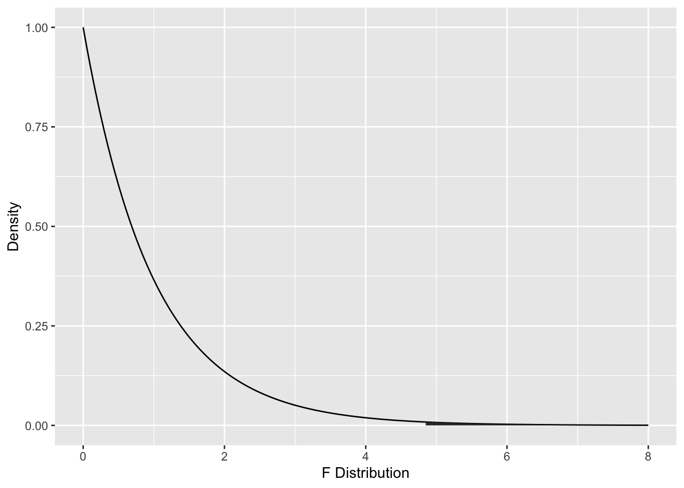
The ANOVA table gives the $p$-value as Pr(>F), here $P = 0.009231$. We could compute this from $F$ using:

pf(4.8269, df1 = 2, df2 = 158, lower.tail = FALSE)

## [1] 0.009231051

According to the $p$-value, we would reject at the $\alpha = .05$ level and conclude that not all three of the groups had the same mean of predicting how strongly Pakistanis felt secondary emotions after the disaster.

11.3.2 Mice on THC

Let’s return to fosdata::mice_pot. We have already seen that the distributions are approximately normal with approximately equal variance, and independence does not seem to be an issue. The null hypothesis is

$H_0: \mu_1 = \cdots = \mu_4$, where $\mu_i$ is the true mean percent activity relative to baseline, and the alternative hypothesis is that at least one of the means is different. We will test at the $\alpha = .05$ level.

To perform ANOVA in R, we first build a linear model of the numeric variable on the grouping variable. Then we run anova on the model object.

mice_mod <- lm(percent_of_act ~ group, data = mice_pot)
anova(mice_mod)

## Analysis of Variance Table
## 
## Response: percent_of_act
##           Df Sum Sq Mean Sq F value Pr(>F)  
## group      3   6329 2109.65  3.1261 0.0357 *
## Residuals 42  28344  674.85                 
## ---
## Signif. codes:  0 '***' 0.001 '**' 0.01 '*' 0.05 '.' 0.1 ' ' 1

We see that we have a $p$-value of $p = .0357$, so we would reject the null hypothesis that all of the means are the same at tha $\alpha = .05$ level.

Recall that it is essential that group be a factor. It is a serious mistake to have the grouping variable as numeric, but R will not give a warning. One good check is that the degrees of freedom should be the number of groups minus 1. If it is 1 and you don’t have two groups, then you likely miscoded the grouping variable.

11.3.3 Chimpanzees (unequal variance)

Consider the data set chimps in the fosdata package. We can load the data via

chimps <- fosdata::chimps

By Ikiwaner - Own work, GFDL 1.2, https://commons.wikimedia.org/w/index.php?curid=11343938

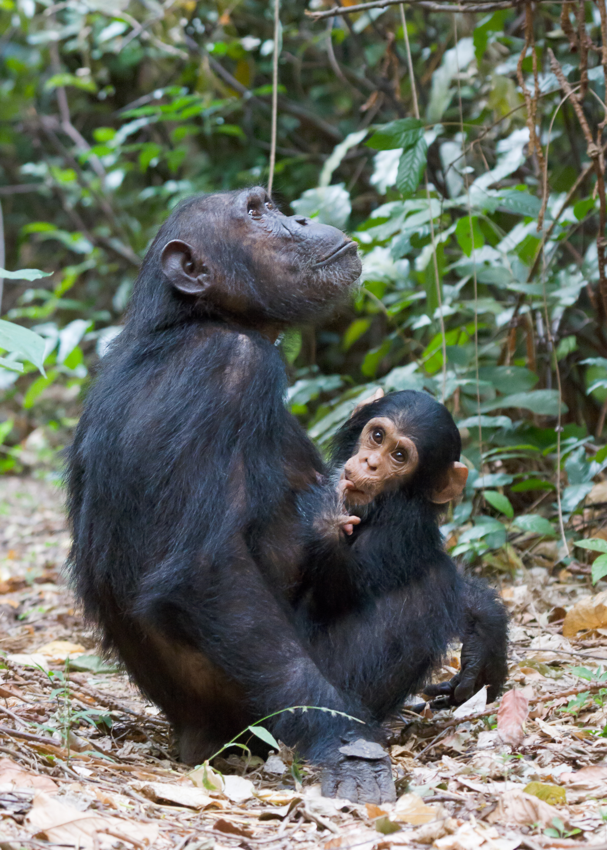
Photographs of chimpanzees of known ages were shown to human judges, who indicated on a scale of 1-6 how gray the chimpanzee’s facial hair was (excluding the chin, which even in juveniles is often gray). The original paper is here ³⁸. The authors’ goal was to determine whether gray hair in chimpanzees increases with age, as it does with humans. The authors found that after age 30, there does not seem to be an age effect.

We will use the data in a different way. We wish to determine whether the mean gray hair is different for chimpanzees 30 or over in the three groups. The authors of the study did not find an age effect, so we wil not account for the ages of the chimpanzees. Let’s look at a boxplot. We note that one of the chimpanzees (Brownface) has two photographs in the data set from when he was over 29. We arbitrarily choose to delete the photograph from when he was older so as to maintain independence. This choice does not affect the conclusions of the following tests.

chimps %>% 
  filter(age > 29, !(individual == "Brownface" & year == 2011)) %>% 
  ggplot(aes(x = population, y = grey_score_avg)) +
  geom_boxplot()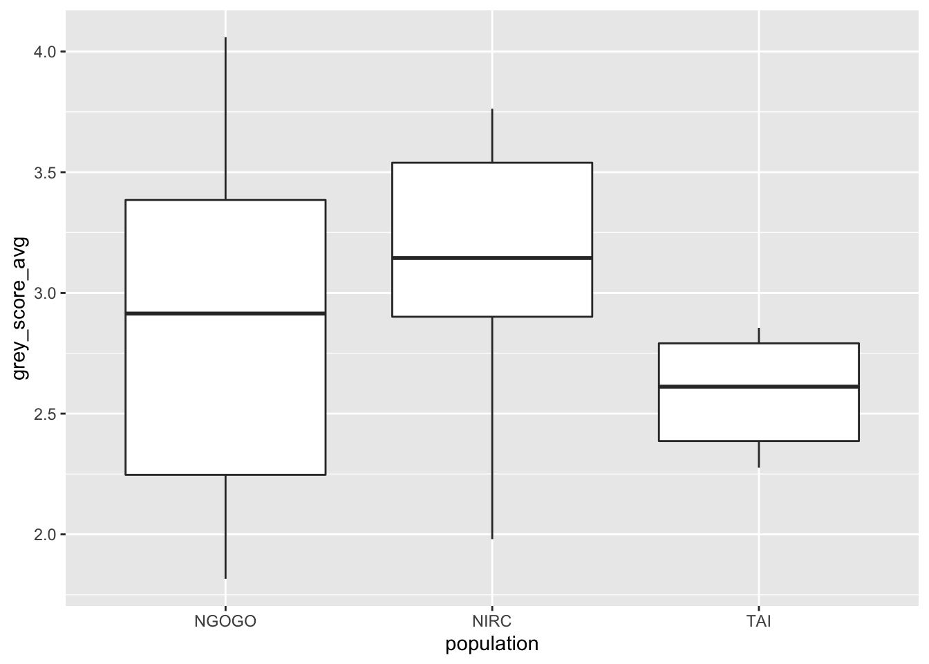

Based on this plot, it appears there may be a difference in mean gray score by population, but it also seems unwise to assume that the variances of the three groups are equal. If we ignore the unequal variances, then we could use anova as follows.

old_chimps <- filter(chimps, age > 29, !(individual == "Brownface" & year == 2011))
chimps_mod <- lm(grey_score_avg ~ population, data = old_chimps)
anova(chimps_mod) #Questionable due to unequal variances

## Analysis of Variance Table
## 
## Response: grey_score_avg
##            Df Sum Sq Mean Sq F value Pr(>F)
## population  2  1.388 0.69402  2.0599 0.1418
## Residuals  37 12.466 0.33692

We would not reject the null hypothesis that the means are the same ($p = .1418$). We will see below that oneway.test is a way to test $H_0: \mu_1 = \cdots = \mu_k$ versus $H_a:$ not all of the $\mu_i$ are equal. It has assumptions of normality in each group, but no assumption of equal variance. Applying oneway.test to this data yields the following.

oneway.test(grey_score_avg ~ population, data = old_chimps)

## 
##  One-way analysis of means (not assuming equal variances)
## 
## data:  grey_score_avg and population
## F = 4.2285, num df = 2.000, denom df = 18.927, p-value = 0.03033

Now, we see that we have a $p$-value of $.03033$, so we would reject $H_0$ that all three groups have the same grayness at the $\alpha = .05$ level. Since equality of variances is a question in this data set, oneway.test is probably the way to go.

11.4 Examining the hypotheses

In this section, we examine the effective type I error rates when $\alpha = .05$ when the underlying populations are normal but have unequal variances. First, let’s look at the equal sample size case. We suppose that we have three groups, two of which have the same variance, and one has a different variance. We examine the effective type I error rates. We fix the number of observations at 30 for each group for now. This piece of code can take a bit of time to run; you might try it with the number of replications equal to 100 or 1000 to start.

variances <- c(.01, .05, .1, .5, 5, 10, 50, 100)

sapply(variances, function(x) {
  sim_data <- replicate(10000, {
  three_groups <- data.frame(group = factor(rep(1:3, each = 30)),
                           values = rnorm(90, 0, rep(c(1, 1, x), each = 30)))
  anova(lm(values ~ group, data = three_groups))$`Pr(>F)`[1]
})
mean(sim_data< .05)
})

## [1] 0.0649 0.0639 0.0608 0.0572 0.0779 0.0866 0.0902 0.0911

We see that when the sample sizes are all equal, and only one group has a different variance, that the group having a large variance tends to make the effective type I error (and more incorrect) larger than when the different group has a smaller variance than the other two groups. Now, what happens if the variance in the third group is larger, and the sample size is different in the third group?

sample_sizes <- c(10, 20, 50, 100, 500)
sapply(sample_sizes, function(x) {
  sim_data <- replicate(1000, {
  three_groups <- data.frame(group = factor(rep(1:3, times = c(30, 30, x))),
                           values = rnorm(60 + x, 0, rep(c(1, 1, 5), times = c(30, 30, x))))
  anova(lm(values ~ group, data = three_groups))$`Pr(>F)`[1]
})
mean(sim_data< .05)
})

## [1] 0.292 0.132 0.021 0.003 0.000

Note that the unequal sample size exacerbates the problem! When the sample size is small relative to the other two, then the effective type I error rate when $\alpha = .05$ is as high as 30 per cent, and when the sample size is large, then the effective type I error rate can get less than 0.001. Now, let’s compare what happens when we use oneway.test.

sample_sizes <- c(10, 20, 50, 100, 500)
sapply(sample_sizes, function(x) {
  sim_data <- replicate(1000, {
  three_groups <- data.frame(group = factor(rep(1:3, times = c(30, 30, x))),
                           values = rnorm(60 + x, 0, rep(c(1, 1, 5), times = c(30, 30, x))))
  oneway.test(values ~ group, data = three_groups)$p.value
})
mean(sim_data< .05)
})

## [1] 0.044 0.059 0.037 0.044 0.053

There doesn’t seem to be any significant issue with oneway.test; the effective type I error rate when $\alpha = .05$ appears to be approximately $.05$, as desired.

In the exercises, you are asked to examine what happens when there are outliers and when one of the groups is skew. If you suspect your populations may not follow the assumptions that we need in order to do ANOVA, you can run some simulations to get a feel for how big of a problem it might be. So, for example, if you had two samples of size 30 and one of size 10, then you would want to be pretty strict about the equal variance assumption. If your sample sizes are all 30, then you don’t need to be as strict.

11.5 Pairwise t-tests and FWER

Suppose we have $k$ groups of observations. Another approach is to do $\binom{k}{2}$ t-tests, and adjust the $p$-values for the fact that we are doing multiple t-tests. This has the advantage of showing directly which pairs of groups have significant differences in means, but the disadvantage of not testing directly $H_0: \mu_1 = \mu_2 = \cdots = \mu_k$ versus $H_a:$ at least one of the means is different. See Exercise 6.

Let’s begin by seeing that we will definitely need to adjust the $p$-values. Suppose we are testing at the $\alpha = .05$ level, and we have $6$ groups of observations all with the same mean. Then, we are doing ${\binom{6}{2}}$ pairs of tests, each of which has a probability of a type I error of $.05$. We cannot really assume that the pairs of tests are independent, because if we know one pair is significantly different, that indicates an increased likelihood that at least one of the groups is different than the others. However, as a first estimate, we can assume independence to get an idea what the probability is of making an error in any of the 15 tests that we are doing. The probability of not making an error is 0.95, so the probability of not making an error in any of the tests is $0.95^{15} \approx 0.46$. Hence, the probability of a type I error in at least one of the tests is $1 - .95^{15} \approx 0.54$. The Family Wide Error Rate is the probability of making at least one type I error in any of the family of tests that are conducted. We have estimated it to be about $0.54$ (assuming independence) in the computation above.

Let’s follow up with some simulations to check. We assume all 6 groups are normal with mean 0 and standard deviation 1. The R command for doing pairwise $t$ tests is pairwise.t.test. The function pairwise.t.test has the following arguments.

x the values of the experiment, or the response vector.
g the grouping of the experiment into populations.
p.adjust.method is the method for adjusting the $p$ values. This includes the options “none”, “holm” and “bonferroni”. Default is “holm”.
pool.sd indicates whether we want to pool the standard deviation across all of the groups to get an estimate of the common standard deviation, or whether we estimate the standard deviation of each group separately. Set to TRUE if we know that the variances of all the groups are equal, or possibly if some of the groups are small. Otherwise, FALSE.

For our purposed for this simulation, we will set p.adjust.method to be “none”, so we can see whether the FWER is about 0.537. Let’s first see what the output looks like.

six_groups <- data.frame(values = rnorm(60),
                         groups = factor(rep(1:6, each = 10)))
pairwise.t.test(six_groups$values,
                six_groups$groups,
                p.adjust.method = "none")

## 
##  Pairwise comparisons using t tests with pooled SD 
## 
## data:  six_groups$values and six_groups$groups 
## 
##   1    2    3    4    5   
## 2 0.42 -    -    -    -   
## 3 0.97 0.44 -    -    -   
## 4 0.50 0.90 0.52 -    -   
## 5 0.23 0.69 0.24 0.59 -   
## 6 0.31 0.83 0.33 0.73 0.85
## 
## P value adjustment method: none

OK, we need to see whether any of the $p$-values are less than 0.05, which would indicate that we would reject the null hypothesis of that pair of means being equal.

any(pairwise.t.test(six_groups$values,
                six_groups$groups,
                p.adjust.method = "none")$p.value < .05, na.rm = TRUE)

## [1] FALSE

Now, we put that inside of replicate.

sim_data <- replicate(10000, {
  six_groups <- data.frame(values = rnorm(60),
                         groups = factor(rep(1:6, each = 10)))
any(pairwise.t.test(six_groups$values,
                six_groups$groups,
                p.adjust.method = "none")$p.value < .05, na.rm = TRUE)
  
})
mean(sim_data)

## [1] 0.3441

We see that our original estimate of $0.54$ was significantly off. The true FWER of the experiment is closer to 0.3441. This indicates that the $p$-values of the tests are not independent. Nonetheless, it is disconcerting that the FWER of the experiment is over 1/3 when we set $\alpha = .05$!

The simplest correction is the Bonferroni correction, which simply multiplies each $p$-value by the number of comparisons being made, rounding down to 1 if necessary. This is a conservative approach, and will lead to a FWER of less than the specified $\alpha$ level. Let’s look at some simulations, where we simply multiply all of the $p$-values by 15, the number of comparisons. We should end up with a FWER of less than 0.05.

sim_data <- replicate(10000, {
  six_groups <- data.frame(values = rnorm(60),
                         groups = factor(rep(1:6, each = 10)))
  any(pairwise.t.test(six_groups$values,
                six_groups$groups,
                p.adjust.method = "bonferroni")$p.value < .05, na.rm = TRUE)
  
})
mean(sim_data)

## [1] 0.0403

We see that our FWER is 0.0403, which is indeed less than $\alpha = .05$. If we use “holm”, then the FWER will still be less than or equal to $\alpha - .05$. In fact, the FWER of “holm” is the same as that of “bonferroni”!

sim_data <- replicate(10000, {
  six_groups <- data.frame(values = rnorm(60),
                         groups = factor(rep(1:6, each = 10)))
  any(pairwise.t.test(six_groups$values,
                six_groups$groups,
                p.adjust.method = "holm")$p.value < .05, na.rm = TRUE)
  
})
mean(sim_data)

## [1] 0.0376

Now, we get an estimate of the FWER as 0.0376, which is indeed less than $\alpha = .05$ and not significantly different than the Bonferroni FWER.

In Exercise @(bonf_holm), you are asked to show that the power of “holm” is higher than the power of “bonferroni” in a specific instance. In general, Holm is at least as powerful as Bonferroni, while having the same FWER, and for this reason is preferred.

Returning to the humanization data, we could do a pairwise t test via the following command. The first argument is the response and the second argument is the grouping variable.

pairwise.t.test(kat_humanization$pak_sec, kat_humanization$group)

## 
##  Pairwise comparisons using t tests with pooled SD 
## 
## data:  kat_humanization$pak_sec and kat_humanization$group 
## 
##              Katrina control Katrina low
## Katrina low  0.033           -          
## Katrina high 0.013           0.647      
## 
## P value adjustment method: holm

We see that there is a significant difference at $\alpha = .05$ between the control and both the low and high levels of aid stories, but no significant difference between the high and low level of aid stories.

pool.sd = TRUE can be used when we are assuming equal variances among the groups, and we want to use all of the groups together to estimate the standard deviation. This can be useful if one of the groups is small, for example, but it does require the assumption that the variances of each group is the same.
p.adjust.method can be set to one of several options, which can be viewed by typing p.adjust.methods. The easiest to understand is “bonferroni”, which multiplies the $p$-values by the number of tests being performed. This is a very conservative adjustment method! The default holm is a good choice. If you wish to compare the results to t.test for diagnostic purposes, then set p.adust.method = "none".
alternative = "greater" or “less” can be used for one sided-tests. Care must be taken to get the order of the groupings correct in this case.
var.equal = TRUE can be used if we know the variances are equal, but we do not want to pool the standard deviation. The default is var.equal = FALSE, just like in t.test. This option is not generally recommended.
If you have common units that are being used across all groups, then one-way ANOVA is not appropriate due to dependence. But, one can still use pairwise.t.test with paired = TRUE. See Exercise @(cowssmall).

Vignette: Reproducibility

Up to this point in the book, we have emphasized writing reproducible code. Ideally, someone could take your R script or R Markdown file and run it as is to get exactly the results that you reported. This is important because it can often be challenging to understand which exact details were used for a statistical test when reading the summary. Having the code available eliminates any confusion about what was done.

A second notion of reproducibility is that of reproducible science. A crucial aspect of the scientific method is that experiments should be reproducible. However, there is currently a reproducibility crisis in several scientific areas, in the sense that it is believed that many published results would not be reproduced if the experiment ran again. Here are some reasons for that.

If you say that a $p$-value less than .05 means that we can reject $H_0$, that means that we will reject $H_0$ five percent of the time even when it is true. Now, consider how many thousands of statistical tests are run each day. It is quite likely that many of the times that $p < .05$ it is simply due to chance. This leads to a problem reproducing significance.
Many experiments do not compute a sample size needed to attain a reasonable power for the test they will be running. What tends to happen in cases where the test is underpowered and yet $p < .05$ is that the effect size gets overestimated. That is, if we are interested not only in whether $H_0$ is false but also how big of a difference from $H_0$ is there, we will overestimate that value in an underpowered test. This leads to a problem reproducing effect sizes. We recommend doing a power analysis whenever possible before collecting data.
Some experimenters will take measurements on hundreds or thousands of variables, and look for interesting significant patterns. If the experimenters do enough tests and check on enough things, then eventually they will find something that is statistically significant. This is fine, as long as the experimenters report all of the tests that they conducted or considered in addition to the ones that were significant. Unethical researchers might not report on the data that wasn’t signifcant, which is an example of $p$-hacking. But even if they report all of the tests that were run, people can be misled by the statistically significant results, and assign it more significance that it deserves. Both of these lead to problems of reproducing significance, but we recommend reporting all tests that were run (or considered, but not run based on the data) on an experiment. We also recommend making all data and scripts public, whenever it is not specifically disallowed for ethical reasons.
Researchers degrees of freedom. There are many decisions that go into analyzing data (not to mention collecting data). Consider outliers. If we think that data is an outlier or may have been miscoded, it is common practice to check with the person who collected the data. How do we decide what appears to be an outlier? If there are too many, then maybe we use a Wilcoxon Rank Sum test or other method that is robust to outliers rather than a $t$-test. If we are using a $t$-test, how do we decide whether var.equal is TRUE or FALSE? Do you do a log transform of the data? Is the alternative hypothesis one-sided or two-sided? There are any number of things that we may or may not do when analyzing a data set, and each one has an effect on the outcome that we normally aren’t sure of. We recommend pre-registering your experiment before starting. Pre-registration involves stating the details of the data collection and analysis procedure before starting to collect data. Any deviance from pre-registration should be noted and justified.
Replication studies are not seen as exciting, so are not conducted as often as they should be. This leads to a paper with problems 1-4 staying unchallenged and uncorrected for too long.

Exercises

Consider the penguins data set in the palmerpenguins package that was discussed in Chapter 10.
1. Create a boxplot of the variable bill_depth_mm by species. Does it appear that the data satisfies the assumptions for ANOVA?
2. Test $H_0$ all of the mean bill depths of the species are the same versus $H_a$ not all of the mean bill depths are the same at the $\alpha = .01$ level.
3. If you reject $H_0$, perform a post-hoc analysis to determine which pairs of mean bill depths are the same, and which are different at the $\alpha = .01$ level.
Consider the frogs data set in the fosdata package. This data set contains measurements from 6 species of frogs, including one new species, dakha, that the authors of the paper found. When establishing that a group of animals is a new species, it can be important to find physiological differences between the group of animals and animals that are nearest genetically. Read more about the data set by typing ?fosdata::frogs.
1. Create a boxplot of the distance from front of eyes to the nostril versus species. Does it appear that the data satisfies the assumptions for ANOVA?
2. Test $H_0$: all of the mean distances of the species are the same versus $H_a$ not all of the mean distances of the species are the same at the $\alpha = .05$ level.
3. IF you reject $H_0$, perform a post-hoc analysis to determine which pairs of mean bill depths are the same, and which are different at the $\alpha = .05$ level. Write up your result in an organized fashion with explanations.
Consider the case0502 data from Sleuth3. Dr Benjamin Spock was tried in Boston for encouraging young men not to register for the draft. It was conjectured that the judge in Spock’s trial did not have appropriate representation of women. The jurors were supposed to be selected by taking a random sample of 30 people (called venires), from which the jurors would be chosen. In the data case0502, the percent of women in 7 judges’ venires are given.
1. Create a boxplot of the percent women for each of the 7 judges. Comment on whether you believe that Spock’s lawyers might have a point.
2. Determine whether there is a significant difference in the percent of women included in the 6 judges’ venires who aren’t Spock’s judge.
3. Determine whether there is a significant difference in the percent of women induced in Spock’s venires versus the percent included in the other judges’ venires combined. (Your answer to b. should justify doing this.)
Consider the data in ex0524 in Sleuth3. This gives 2584 data points, where the subjects’ IQ was measured in 1979 and their Income was measured in 2005. Create a boxplot of income for each of the IQ quartiles. Is there evidence to suggest that there is a difference in mean income among the 4 groups of IQ? Check the residuals in your model. Does this cause you to doubt your result?
The built in data set InsectSprays records the counts of living insects in agricultural experimental units treated with different insecticides.
1. Plot the data. Three of the sprays seem to be more effective (less insects collected) than the other three sprays. Which three are the more effective sprays?
2. Use ANOVA to test if the three effective sprays have the same mean. What do you conclude?
3. Use ANOVA to test if the three less effective sprays have the same mean. What do you conclude?
4. Would it be appropriate to use ANOVA on the entire data set? Why or why not?
5. Use oneway.test to test the null hypothesis that all of the mean insect counts are the same for the various sprays versus the alternative that they are not, at the $\alpha = .01$ level.
The built in data set chickwts measures weights of chicks after six weeks eating various types of feed. Test if the the mean weight is the same for all feed types. Check the residuals - are the assumptions for ANOVA reasonable?
The data set MASS::immer from the MASS package has data on a trial of barley varieties performed by Immer, Hayes, and Powers in the early 1930’s. Test if the total yield (sum of 1931 and 1932) depends on the variety of barley. Check the residuals - are the assumptions for ANOVA reasonable?
The built in data set morley gives speed of light measurements for five experiments done by Michelson in 1879.
1. Create a boxplot with one box for each of the five experiments.
2. Use ANOVA to test if the five experiments have the same mean. What do you conclude?
Suppose you have 6 groups of 15 observations each. Groups 1-3 are normal with mean 0 and standard deviation 3, while groups 4-6 are normal with mean 1 and standard deviation 3. Compare via simulation the power of the following tests of $H_0: \mu_1 = \cdot = \mu_6$ versus the alternative that at least one pair is different at the $\alpha = .05$ level.
1. ANOVA. (Hint: anova(lm(formula, data))[1,5] pulls out the p-value of ANOVA.)
2. pairwise.t.test, where we reject the null hypothesis if any of the paired $p$-values are less than 0.05.
Suppose you have three populations, all of which are normal with standard deviation 1, and with means $0$, $0.5$ and $1$. You take samples of size 30 and perform a pairwise $t$ test.
1. Estimate the percentage of times that the null hypotheses being tested are rejected when using the “bonferroni” $p$-value adjustment.
2. Estimate the percentage of times that the null hypotheses being tested are rejected when using the “holm” $p$-value adjustment.
Consider the data set cows_small in the fosdata package. In this data set, cows in Davis, CA were sprayed with water on hot days to try to cool them down. Each cow was measured with no spray (control), nozzle TK-0.75, and nozle TK-12.
1. Is one-way ANOVA appropriate to use on this data set? If so, do it. If not, explain why not.
2. Perform pairwise $t$ tests on the three groups with holm $p$-value adjustment and explain.

Viñals X, Moreno E, Lanfumey L, Cordomí A, Pastor A, de La Torre R, et al. (2015) Cognitive Impairment Induced by Delta9-tetrahydrocannabinol Occurs through Heteromers between Cannabinoid CB1 and Serotonin 5-HT2A Receptors. PLoS Biol 13(7): e1002194. https://doi.org/10.1371/journal.pbio.1002194 ↩︎
Tapanes E, Anestis S, Kamilar JM, Bradley BJ (2020) Does facial hair greying in chimpanzees provide a salient progressive cue of aging? PLoS ONE 15(7): e0235610. https://doi.org/10.1371/journal.pone.0235610 ↩︎