Chapter 12 Multiple Regression
In this short chapter, we consider the case where we have a single numeric response variable, and multiple explanatory variables. There is a natural tension between explaining the response and having a simple model. Our main purpose will be to understand this tension and find a balance between the two competing goals.
12.1 Two explanatory variables
We consider housing data from King County, WA, which includes Seattle. The data includes various properties of houses and their sale price. Our goal is to model the sale price on the other variables. There are many variables that we could use to do this, but in this section we will only consider two of them; namely, the square footage in the house and the size of the lot in ZIP code 98103. The data set is houses in the fosdata package.
We first need to filter out only those houses that are in ZIP code 98103, and we will only be using the price, sqft_living and sqft_lot variables, so we will select those columns.
See that there are now 602 observations. We start by doing some summary statistics and visualizations.
##      price          sqft_living      sqft_lot
##  Min.   : 238000   Min.   : 390   Min.   : 651
##  1st Qu.: 432125   1st Qu.:1242   1st Qu.:1563
##  Median : 550000   Median :1505   Median :3500
##  Mean   : 584919   Mean   :1651   Mean   :3482
##  3rd Qu.: 695000   3rd Qu.:1960   3rd Qu.:4800
##  Max.   :1695000   Max.   :4360   Max.   :9450
It appears that the variables may be right-skew based on that. Let’s compute the skewness:
##       price sqft_living    sqft_lot
##   1.3948617   1.2411793   0.4180971
The variables price and sqft_living are right-skew and the variable sqft_lot is moderately right-skew. Let’s look at histograms and scatterplots.
library(tidyr) # for pivot_longer
houses_98103 %>%
  pivot_longer(cols = c(price, sqft_living, sqft_lot)) %>%
  ggplot(aes(value)) +
  geom_histogram(bins = 15) +
  facet_wrap(~name, scales = "free_x")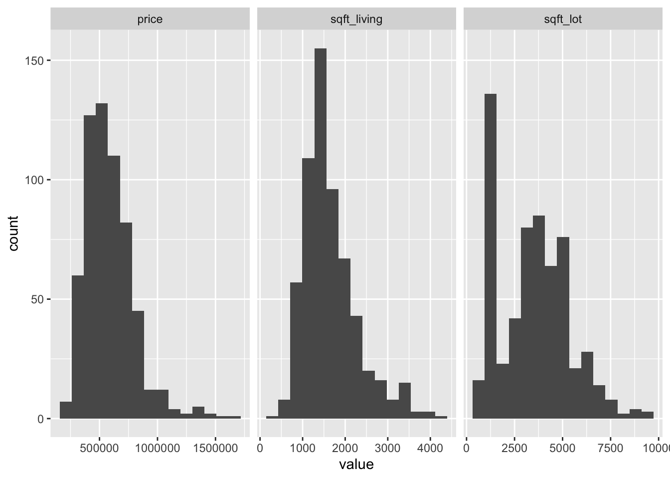
Now let’s look at three scatterplots.
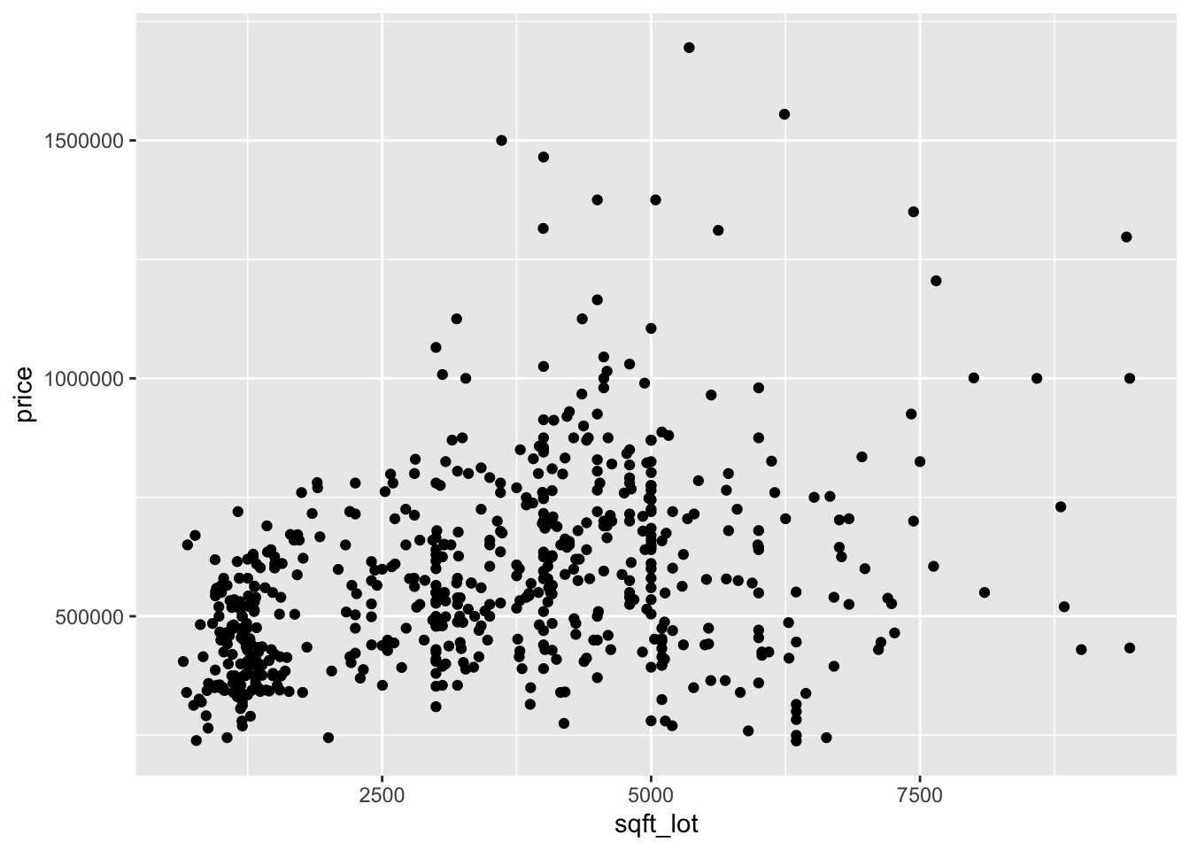
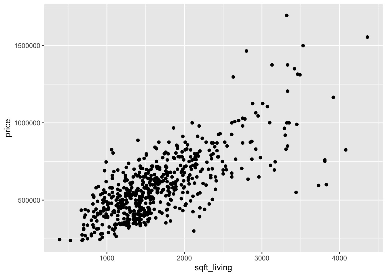
Looking at the two plots separately, it appears that the variance of price is not constant across the explanatory variables. Combining this with the fact that the variables are skew, we re-plot the scatterplots with logs.
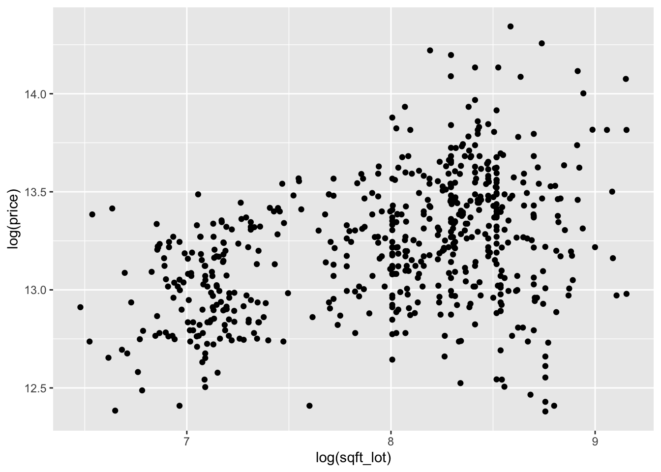
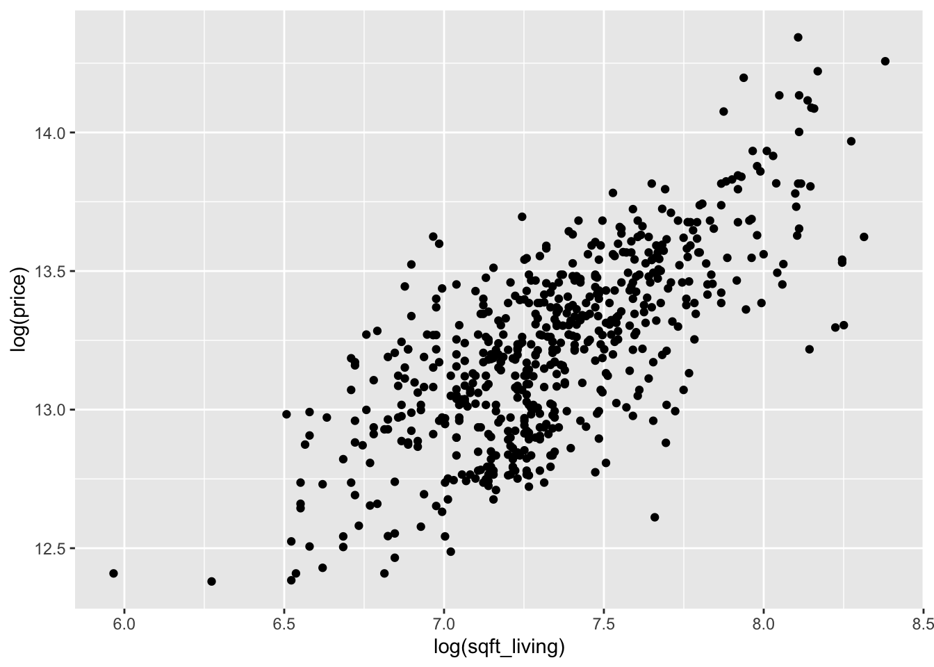
We continue by modeling the log of price on the log of the two explanatory variables. With only two explanatory variables, it is still possible to visualize the relationship. For scatterplots in three dimensions, we recommend plotly. We will not be utilizing all of the features of plotly, so we do not go into detail.
plotly::plot_ly(houses_98103,
  x = ~ log(houses_98103$sqft_living),
  y = ~ log(houses_98103$sqft_lot),
  z = ~ log(houses_98103$price),
  type = "scatter3d"
)
Looking at the scatterplot, it seems reasonable that a plane could model the relationship between \(x\), \(y\) and \(z\). How would we find the equation of the plane that is the best fit? Well, a plane has an equation of the form \(ax + by + cz = d\), and we are assuming that there is some dependence on \(z\), so \(c\not=0\). Therefore, we can write the equation of the plane as \(z = \beta_0 + \beta_1 x + \beta_2 y\) for some choices of \(\beta_0, \beta_1\) and \(\beta_2\). (In terms of the original equation, \(\beta_0 = d/c,\, \beta_1 = -b/c,\, \beta_2 = -a/c\).) For each \(\beta_0, \beta_1\) and \(\beta_2\) we can predict the values of \(z\) at the values of the explanatory variables by computing \(\hat z_i = \beta_0 + \beta_1 x_i + \beta_2 y_i\). The associated error is \(\hat z_i - z_i\), and we find the values of \(\beta_0, \beta_1\) and \(\beta_2\) that minimize the sum of squares of the error.
Model: Our model is \[ z_i = \beta_0 + \beta_1 x_i + \beta_2 y_i + \epsilon_i \] where \(\beta_0, \beta_1\) and \(\beta_2\) are unknown constants, and \(\epsilon_i\) are independent, identically distributed normal random variables. The \(i\)th response is given by \(z_i\), and the \(i\)th predictors are \(x_i\) and \(y_i\).
For example, if \(\beta_0 = \beta_1 = \beta_2 = 1\), then we can compute the sum of squared error via
sum((1 + 1 * log(houses_98103$sqft_living) +
       1 * log(houses_98103$sqft_lot) -
       log(houses_98103$price))^2)
## [1] 6066.812We can find the values of \(\beta_0, \beta_1\) and \(\beta_2\) that minimize the SSE using lm. The format is very similar to the single explanatory variable case.
##
## Call:
## lm(formula = log(price) ~ log(sqft_living) + log(sqft_lot), data = houses_98103)
##
## Residuals:
##      Min       1Q   Median       3Q      Max
## -0.89008 -0.16904  0.02388  0.16157  0.58681
##
## Coefficients:
##                  Estimate Std. Error t value Pr(>|t|)
## (Intercept)       7.83039    0.19607  39.937  < 2e-16 ***
## log(sqft_living)  0.61291    0.02636  23.252  < 2e-16 ***
## log(sqft_lot)     0.11156    0.01535   7.265 1.16e-12 ***
## ---
## Signif. codes:  0 '***' 0.001 '**' 0.01 '*' 0.05 '.' 0.1 ' ' 1
##
## Residual standard error: 0.223 on 599 degrees of freedom
## Multiple R-squared:  0.5598, Adjusted R-squared:  0.5583
## F-statistic: 380.8 on 2 and 599 DF,  p-value: < 2.2e-16
We ignore most of the output for now, and focus on the estimates of the coefficients. Namely, \(\beta_0 = 7.83039\), \(\beta_1 = 0.61291\) and \(\beta_2 = 0.11156\). For comparison, these coefficients lead to a SSE of
sum((7.83039 +
  0.61291 * log(houses_98103$sqft_living) +
  0.11156 * log(houses_98103$sqft_lot) -
  log(houses_98103$price))^2)
## [1] 29.78089which is much smaller than the original value that we computed above! The interested reader can check that if they change any of the coefficients by some small amount, then the SSE computed above will increase. Let’s use plotly one last time to visualize the plane. We include the code for completeness, but do not explain the details of how to do this. Plotly produces interactive plots that do not render well on paper, so we recommend running this code in R to see the results.
library(tibble) # for column_to_rownames
xs <- seq(min(log(houses_98103$sqft_living) - 1),
  max(log(houses_98103$sqft_living) + 1),
  length.out = 30
)
ys <- seq(min(log(houses_98103$sqft_lot)) - 1,
  max(log(houses_98103$sqft_lot)) + 1,
  length.out = 30
)
grid <- expand.grid(xs, ys)
grid <- mutate(grid,
  surface = 7.830385 + 0.6129149 * Var1 + 0.1115567 * Var2
)
z <- pivot_wider(grid, names_from = Var2, values_from = surface) %>%
  column_to_rownames(var = "Var1")
z <- as.matrix(z)plotly::plot_ly(houses_98103,
x = ~ log(sqft_lot),
y = ~ log(sqft_living),
z = ~ log(price),
type = "scatter3d"
) %>%
plotly::add_markers() %>%
plotly::add_trace(
z = z,
x = xs,
y = ys,
type = "surface",
inherit = T
)Let’s now examine the summary of lm when there are two explanatory variables. We will go through line by line, much as we did in the previous chapter, to explain what each value represents.
##
## Call:
## lm(formula = log(price) ~ log(sqft_living) + log(sqft_lot), data = houses_98103)
##
## Residuals:
##      Min       1Q   Median       3Q      Max
## -0.89008 -0.16904  0.02388  0.16157  0.58681
##
## Coefficients:
##                  Estimate Std. Error t value Pr(>|t|)
## (Intercept)       7.83039    0.19607  39.937  < 2e-16 ***
## log(sqft_living)  0.61291    0.02636  23.252  < 2e-16 ***
## log(sqft_lot)     0.11156    0.01535   7.265 1.16e-12 ***
## ---
## Signif. codes:  0 '***' 0.001 '**' 0.01 '*' 0.05 '.' 0.1 ' ' 1
##
## Residual standard error: 0.223 on 599 degrees of freedom
## Multiple R-squared:  0.5598, Adjusted R-squared:  0.5583
## F-statistic: 380.8 on 2 and 599 DF,  p-value: < 2.2e-16
lm(formula = log(price) ~ log(sqft_living) + log(sqft_lot), data = houses_98103)this gives the call tolmthat was used to create the model. It can be useful when you are comparing multiple models, or when a function creates a model for you without your typing it in directly.ResidualsThis gives the values of the estimated value of the response minus the actual value of the response. Many times, we will assume a model of \(y = \beta_0 + \beta_1 x + \beta_2 y + \epsilon\), where \(\epsilon\) is normal. In this case, we should expect that the residuals are symmetric about 0, so we would like to see that the median is about 0, the 1st and 3rd quartiles are about equal, and the min and max are about equal.CoefficientsThis gives the estimate for the coefficients, together with the standard error, \(t\)-value for use in a t-test of significance, and \(p\)-value. The \(p\)-value is for the test of \(H_0: \beta_i = 0\) versus \(H_a: \beta_i \not= 0\). In this instance, we reject the null hypotheses that the two slopes and intercept are zero. The \(\epsilon_i\) must be normal in order for these \(p\)-values to be accurate.Residual standard error. This can be computed from the residuals as follows:
## [1] 0.2229746Recall our rule of thumb that we divide by the sample size minus the number of estimated parameters when estimating \(\sigma\). In this case, there are three estimated parameters. The degrees of freedom is just the number of samples minus the number of parameters estimated.
Multiple R-squaredcan be interpreted as the percent of variance in the response that is explained by the model. It can be computed as follows:
var_response <- var(log(houses_98103$price))
var_residuals <- var(residuals(mod))
(var_response - var_residuals) / var_response
## [1] 0.5597819The Adjusted \(R^2\) uses the residual standard error (that has been adjusted for the number of parameters) rather than the raw variance of the residuals.
## [1] 0.5583121The multiple \(R^2\) value will increase with the addition of more variables, where the adjusted \(R^2\) has a penalty for adding variables, so can either increase of decrease when a new variable is added.
F statisticthis is the test statistic used to test \(H_0: \beta_1 = \beta_2 = \cdots = 0\) versus not all of the slopes are 0. Note this does not include a test for the intercept. The \(\epsilon_i\) must be normal for this to be accurate. We compute the value via
N <- nrow(houses_98103)
ssresid <- sum(residuals(mod)^2)
ssresponse <- sum((log(houses_98103$price) - mean(log(houses_98103$price)))^2)
(ssresponse - ssresid) / 2 / (ssresid / (N - 3))
## [1] 380.844612.2 Categorical Variables
In this section we briefly explain hos R treats categorical variables in lm via an example. Let’s expand the ZIP codes in our model to include three different ones.
We again take the log of price, sqft_lot and sqft_living.
houses_3zips <- mutate(houses_3zips,
  sqft_lot = log(sqft_lot),
  sqft_living = log(sqft_living),
  price = log(price)
)
houses_3zips$zipcode <- factor(houses_3zips$zipcode)
ggplot(houses_3zips, aes(x = sqft_living, y = price, color = zipcode)) +
  geom_point() +
  geom_smooth(method = "lm")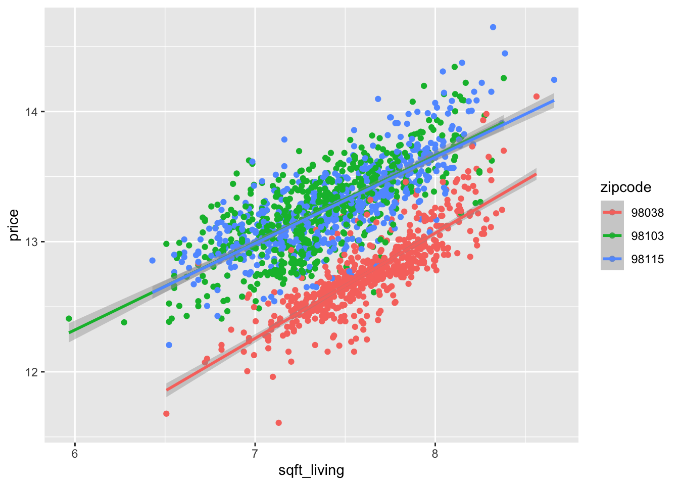
Based on this plot, it appears that 98115 and 98103 have similar characteristics, but 98038 has a different relationship between the log of price and the log of square feet of living space. In particular, while it appears that the slope may be the same, the intercept appears to be different. Let’s see how that pans out in lm.
Note that it would be a mistake to treat zipcode as a numeric variable! We changed it to a factor above.
##
## Call:
## lm(formula = price ~ sqft_living + sqft_lot + zipcode, data = houses_3zips)
##
## Residuals:
## Min 1Q Median 3Q Max
## -0.98317 -0.11125 0.00604 0.11678 0.68475
##
## Coefficients:
## Estimate Std. Error t value Pr(>|t|)
## (Intercept) 6.93118 0.10648 65.09 <2e-16 ***
## sqft_living 0.65761 0.01362 48.27 <2e-16 ***
## sqft_lot 0.08922 0.00629 14.19 <2e-16 ***
## zipcode98103 0.74935 0.01373 54.56 <2e-16 ***
## zipcode98115 0.69703 0.01243 56.09 <2e-16 ***
## ---
## Signif. codes: 0 '***' 0.001 '**' 0.01 '*' 0.05 '.' 0.1 ' ' 1
##
## Residual standard error: 0.1994 on 1770 degrees of freedom
## Multiple R-squared: 0.7537, Adjusted R-squared: 0.7532
## F-statistic: 1354 on 4 and 1770 DF, p-value: < 2.2e-16This says that all three variables are statistically significant. The way to interpret the zipcode coefficients is as follows. There is a “base” level of the factor, which can be obtained by typing levels(house$zipcode). The level that appears first is the “base” level. This means that if we have a house in ZIP code 98038 (the base level), we can compute its estimated log of price via 6.93 + 0.676 * sqft_living + 0.089 * sqft_lot. However, if we wish to compute the log price of a house in ZIP Code 98103, we would compute 6.93 + 0.676 * sqft_living + 0.089 * sqft_lot + 0.74935. That is, there is an additive adjustment that needs to be made when the house is in ZIP code 98103 rather than in 98038.
If you want to change the base level, you can do that as follows.
houses_3zips$zipcode <- factor(houses_3zips$zipcode, levels = c("98103", "98038", "98115"))
mod <- lm(price ~ sqft_living + sqft_lot + zipcode, data = houses_3zips)
summary(mod)
##
## Call:
## lm(formula = price ~ sqft_living + sqft_lot + zipcode, data = houses_3zips)
##
## Residuals:
## Min 1Q Median 3Q Max
## -0.98317 -0.11125 0.00604 0.11678 0.68475
##
## Coefficients:
## Estimate Std. Error t value Pr(>|t|)
## (Intercept) 7.68052 0.10110 75.971 < 2e-16 ***
## sqft_living 0.65761 0.01362 48.272 < 2e-16 ***
## sqft_lot 0.08922 0.00629 14.186 < 2e-16 ***
## zipcode98038 -0.74935 0.01373 -54.562 < 2e-16 ***
## zipcode98115 -0.05232 0.01200 -4.362 1.37e-05 ***
## ---
## Signif. codes: 0 '***' 0.001 '**' 0.01 '*' 0.05 '.' 0.1 ' ' 1
##
## Residual standard error: 0.1994 on 1770 degrees of freedom
## Multiple R-squared: 0.7537, Adjusted R-squared: 0.7532
## F-statistic: 1354 on 4 and 1770 DF, p-value: < 2.2e-16Here we see that there is even a statistically significant difference between ZIP code 98115 and 98103 (the base).
12.3 Variable Selection
One of the goals of linear regression is to be able to choose a parsimonious set of explanatory variables. There are many ways of achieving that, and we present one using \(p\)-values in this section. We consider the data set conversation , which is in the fosdata package adapted from this article.
This study had 210 university students participate in a 10 minute conversation in small groups. The participants also provided various demographic information, and took a test to indicate whether they suffered from subclinical psychopathy. The goal was to determine whether and/or how conversational items such as the proportion of words spoken depend on the demographic data. You can read how the authors of the study analyzed the data in the paper linked above. For us, we want to use this data set to illustrate variable selection, so we are going to model the proportion of words spoken on the variables in the data set. The variables split naturally into two groups: demographic data and conversational data. The conversational data measures the number of interruptions, the number of times that a person started a new topic on a per word basis, and the proportion of times a person started a new topic. The demographic data includes data on shirt type, gender, median income of major, prestige of major, fighting ability (as estimated based on a picture), etc.
A few things to notice about this data set. First, the character data should be encoded as factors, as should gender.
converse$oldest <- factor(converse$oldest)
converse$gender <- factor(converse$gender)
summary(converse)
We do not print out the entire summary, but you can see that many of the variables have been standardized, so as to have approximately mean 0 and standard deviation 1, and that oldest has 72 missing values. We need to decide what to do with that variable, but since it isn’t well documented in the paper, let’s just remove it. We also remove all of the information related to the prisoner’s dilemma part of the experiment. That part of the experiment by necessity happened after the conversations, so it seems to make more sense to model the prisoner’s dilemma outcomes on the conversation than the other way around.
Let’s examine some plots. Here, we pick a few of the explanatory variables to plot versus the response.
ggplot(converse, aes(x = f1_psychopathy, y = proportion_words)) +
  geom_point() +
  geom_smooth(method = "lm")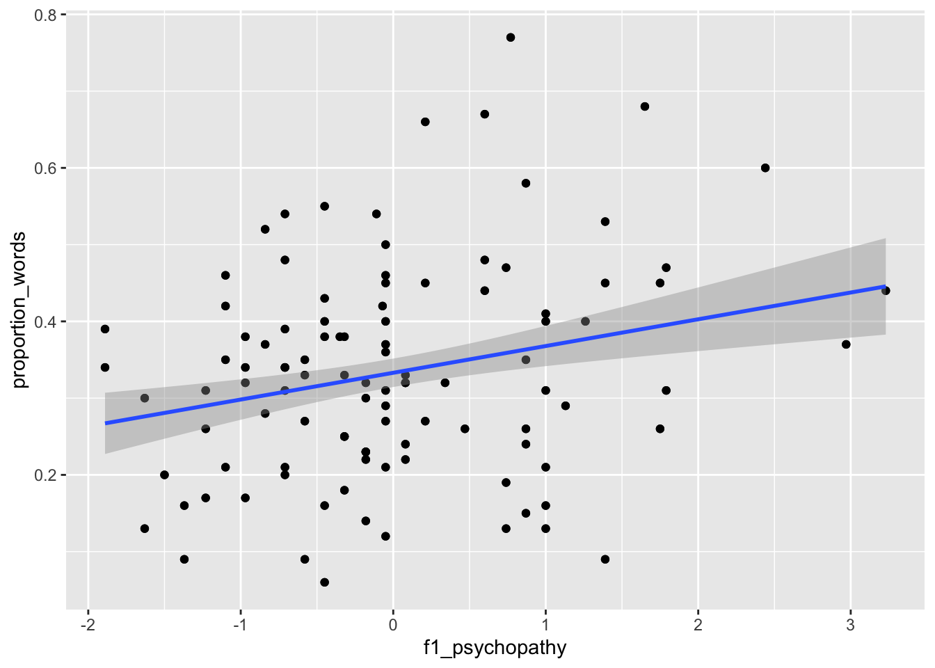
ggplot(converse, aes(x = interruptions_per_min, y = proportion_words)) +
  geom_point() +
  geom_smooth(method = "lm")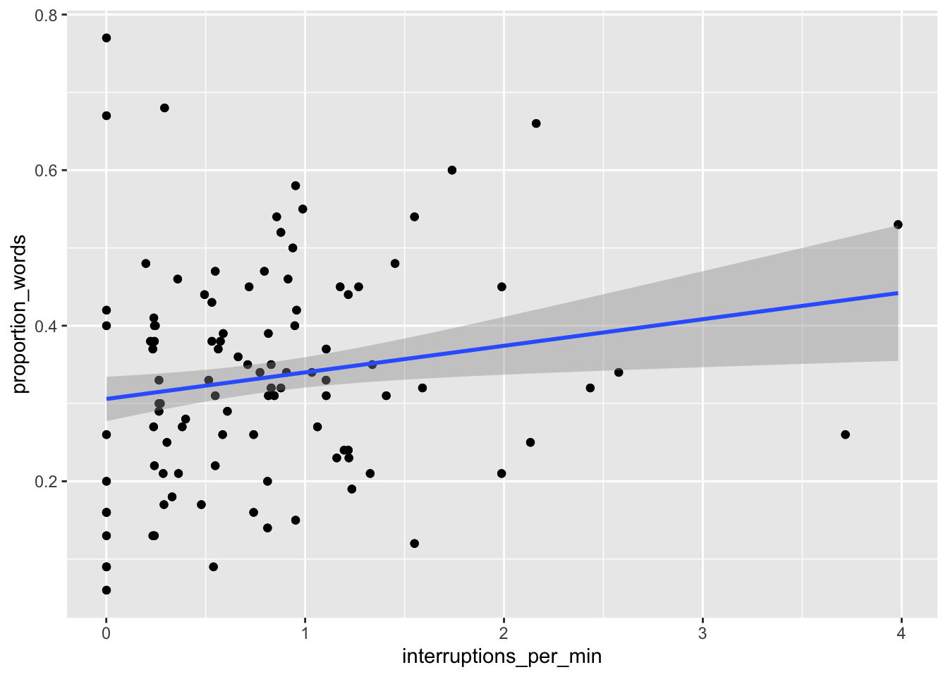
We can see that neither of the two above variables have strong predictive ability for the response by themselves, but perhaps with all of the variables, things will look better.
##
## Call:
## lm(formula = proportion_words ~ ., data = converse)
##
## Residuals:
##       Min        1Q    Median        3Q       Max
## -0.183163 -0.040952  0.002491  0.044088  0.188120
##
## Coefficients:
##                                 Estimate Std. Error t value Pr(>|t|)
## (Intercept)                    0.2959771  0.0305151   9.699  < 2e-16 ***
## gender1                        0.0051863  0.0118649   0.437  0.66252
## f1_psychopathy                -0.1579680  0.4577533  -0.345  0.73040
## f2_psychopathy                -0.0980854  0.2457922  -0.399  0.69029
## total_psychopathy              0.2237067  0.5963622   0.375  0.70799
## attractiveness                -0.0022099  0.0055057  -0.401  0.68859
## fighting_ability              -0.0286368  0.0086793  -3.299  0.00115 **
## strength                       0.0186639  0.0085663   2.179  0.03057 *
## height                        -0.0057262  0.0055482  -1.032  0.30333
## median_income                  0.0001271  0.0002090   0.608  0.54379
## highest_class_rank             0.0242887  0.0115059   2.111  0.03607 *
## major_presige                 -0.0005630  0.0005683  -0.991  0.32313
## dyad_status_difference        -0.0178477  0.0070620  -2.527  0.01230 *
## proportion_sequence_starts     0.4855446  0.0409178  11.866  < 2e-16 ***
## interruptions_per_min          0.1076160  0.0144719   7.436 3.35e-12 ***
## sequence_starts_per_word_x100 -0.0493571  0.0061830  -7.983 1.28e-13 ***
## interruptions_per_word_x100   -0.0708835  0.0094431  -7.506 2.22e-12 ***
## affect_words                  -0.0039201  0.0027227  -1.440  0.15155
## ---
## Signif. codes:  0 '***' 0.001 '**' 0.01 '*' 0.05 '.' 0.1 ' ' 1
##
## Residual standard error: 0.07303 on 192 degrees of freedom
## Multiple R-squared:  0.751,  Adjusted R-squared:  0.729
## F-statistic: 34.07 on 17 and 192 DF,  p-value: < 2.2e-16
A couple of things to notice. First, two of the other three conversation variables are significant when predicting the proportion of words spoken. Second, the multiple \(R^2\) is .751, which means that about 75 percent of the variance in the proportion of words spoken is explained by the explanatory variables. Let’s start removing variables in groups. First, we have the three psychopathy variables. We start by removing them one at a time. We will use the update command, which takes as its first argument the model that we are updating, and the argument is the update that we are making. The form of the second argument we will be using is ~ . - variable_name. For reasons of space, we do not show the entire output at each step. You won’t need to do this when doing your own analysis.
mod2 <- update(mod, ~ . - f1_psychopathy)
mod2 %>%
  broom::tidy() %>%
  mutate(across(where(is.numeric), ~ round(., 3))) %>%
  filter(stringr::str_detect(term, "psycho|Inter")) %>%
knitr::kable()| term | estimate | std.error | statistic | p.value |
|---|---|---|---|---|
| (Intercept) | 0.295 | 0.030 | 9.745 | 0.000 |
| f2_psychopathy | -0.013 | 0.008 | -1.656 | 0.099 |
| total_psychopathy | 0.018 | 0.009 | 2.102 | 0.037 |
## [1] 0.7508613## [1] 0.7302073We see that after removing f1_psychopathy, the variabletotal_psychopathy has coefficient significantly different from 0 (\(p = .037\)), while f2_psychopathy is not significant at the \(\alpha = .05\) level. Also, note that the \(R^2\) did not decrease much when we removed f1_psychopathy, and the adjusted \(R^2\) increased from .729 to .730.. These are good signs that it is OK to remove f1_psychopathy. It is common to see large changes in significance when removing variables that are linked or correlated in some way. We continue removing the variables linked to psychopathy. So, we leave those two variables in for now, and continue removing variables. It seems that gender can be removed.
mod3 <- update(mod2, ~ . - f2_psychopathy)
mod3 %>%
  broom::tidy() %>%
  mutate(across(where(is.numeric), ~ round(., 3))) %>%
  filter(stringr::str_detect(term, "psycho|Inter")) %>%
knitr::kable()| term | estimate | std.error | statistic | p.value |
|---|---|---|---|---|
| (Intercept) | 0.296 | 0.030 | 9.731 | 0.000 |
| total_psychopathy | 0.007 | 0.006 | 1.293 | 0.198 |
## [1] 0.7473232## [1] 0.7277863Here we get conflicting information about whether to remove f2_psychopathy. The variable was not significant at the \(\alpha = .05\) level, but the adjusted \(R^2\) decreases from .730 to .728 when we remove the variable. Different variable selection techniques would do different things at this point. However, we are using \(p\)-values right now, so we continue by removing the last of the psychopathy variables (since it is not significant).
##
## Call:
## lm(formula = proportion_words ~ gender + attractiveness + fighting_ability +
##     strength + height + median_income + highest_class_rank +
##     major_presige + dyad_status_difference + proportion_sequence_starts +
##     interruptions_per_min + sequence_starts_per_word_x100 + interruptions_per_word_x100 +
##     affect_words, data = converse)
##
## Residuals:
##       Min        1Q    Median        3Q       Max
## -0.180736 -0.038420 -0.000994  0.043020  0.202987
##
## Coefficients:
##                                 Estimate Std. Error t value Pr(>|t|)
## (Intercept)                    0.2933090  0.0303800   9.655  < 2e-16 ***
## gender1                       -0.0037965  0.0108581  -0.350 0.726983
## attractiveness                -0.0028329  0.0055096  -0.514 0.607706
## fighting_ability              -0.0304228  0.0083761  -3.632 0.000359 ***
## strength                       0.0211761  0.0083132   2.547 0.011628 *
## height                        -0.0082203  0.0053578  -1.534 0.126585
## median_income                  0.0001295  0.0002088   0.620 0.535722
## highest_class_rank             0.0244283  0.0114397   2.135 0.033976 *
## major_presige                 -0.0004255  0.0005441  -0.782 0.435162
## dyad_status_difference        -0.0153037  0.0069836  -2.191 0.029610 *
## proportion_sequence_starts     0.5013595  0.0399347  12.554  < 2e-16 ***
## interruptions_per_min          0.1138530  0.0141768   8.031 8.97e-14 ***
## sequence_starts_per_word_x100 -0.0481660  0.0061777  -7.797 3.73e-13 ***
## interruptions_per_word_x100   -0.0731355  0.0093695  -7.806 3.53e-13 ***
## affect_words                  -0.0050216  0.0026643  -1.885 0.060946 .
## ---
## Signif. codes:  0 '***' 0.001 '**' 0.01 '*' 0.05 '.' 0.1 ' ' 1
##
## Residual standard error: 0.07331 on 195 degrees of freedom
## Multiple R-squared:  0.7451, Adjusted R-squared:  0.7268
## F-statistic: 40.72 on 14 and 195 DF,  p-value: < 2.2e-16
The adjusted \(R^2\) fell again, this time to .727. Now that we have removed all of the variables related to psychopathy, we can check to see whether as a group they are significant. That is, we will test \(H_0\) the coefficients of the psychopathy variables are all 0 versus \(H_a\) not all of the coefficients are zero.
## Analysis of Variance Table
##
## Model 1: proportion_words ~ gender + attractiveness + fighting_ability +
##     strength + height + median_income + highest_class_rank +
##     major_presige + dyad_status_difference + proportion_sequence_starts +
##     interruptions_per_min + sequence_starts_per_word_x100 + interruptions_per_word_x100 +
##     affect_words
## Model 2: proportion_words ~ gender + f1_psychopathy + f2_psychopathy +
##     total_psychopathy + attractiveness + fighting_ability + strength +
##     height + median_income + highest_class_rank + major_presige +
##     dyad_status_difference + proportion_sequence_starts + interruptions_per_min +
##     sequence_starts_per_word_x100 + interruptions_per_word_x100 +
##     affect_words
##   Res.Df    RSS Df Sum of Sq      F Pr(>F)
## 1    195 1.0481
## 2    192 1.0240  3  0.024138 1.5087 0.2136
We get a \(p\)-value of .2136, so we do not reject the null hypothesis that all of the coefficients are zero. If we had rejected the null hypothesis, then we would have needed to add back in one or more of the variables to the model. It is important when doing stepwise variable selection that you periodically check to see whether you need to add back in one or more of the variables that you removed. Next, we remove the variables that describe the person, such as attractiveness or strength. Again, we go in order of \(p\)-values within that group of variables.
mod5 <- update(mod4, ~ . - gender)
mod6 <- update(mod5, ~ . - attractiveness)
mod7 <- update(mod6, ~ . - median_income)
summary(mod7)
##
## Call:
## lm(formula = proportion_words ~ fighting_ability + strength +
## height + highest_class_rank + major_presige + dyad_status_difference +
## proportion_sequence_starts + interruptions_per_min + sequence_starts_per_word_x100 +
## interruptions_per_word_x100 + affect_words, data = converse)
##
## Residuals:
## Min 1Q Median 3Q Max
## -0.181215 -0.037676 -0.000914 0.042230 0.202280
##
## Coefficients:
## Estimate Std. Error t value Pr(>|t|)
## (Intercept) 0.3024526 0.0214860 14.077 < 2e-16 ***
## fighting_ability -0.0300948 0.0082729 -3.638 0.000351 ***
## strength 0.0207458 0.0082203 2.524 0.012397 *
## height -0.0080111 0.0052692 -1.520 0.130012
## highest_class_rank 0.0243218 0.0112871 2.155 0.032382 *
## major_presige -0.0004917 0.0005239 -0.939 0.349084
## dyad_status_difference -0.0144526 0.0067093 -2.154 0.032439 *
## proportion_sequence_starts 0.5008202 0.0393863 12.716 < 2e-16 ***
## interruptions_per_min 0.1127051 0.0138752 8.123 4.81e-14 ***
## sequence_starts_per_word_x100 -0.0488678 0.0060006 -8.144 4.22e-14 ***
## interruptions_per_word_x100 -0.0725000 0.0092657 -7.825 2.99e-13 ***
## affect_words -0.0048069 0.0025190 -1.908 0.057807 .
## ---
## Signif. codes: 0 '***' 0.001 '**' 0.01 '*' 0.05 '.' 0.1 ' ' 1
##
## Residual standard error: 0.07289 on 198 degrees of freedom
## Multiple R-squared: 0.7442, Adjusted R-squared: 0.73
## F-statistic: 52.37 on 11 and 198 DF, p-value: < 2.2e-16## Analysis of Variance Table
##
## Model 1: proportion_words ~ fighting_ability + strength + height + highest_class_rank +
## major_presige + dyad_status_difference + proportion_sequence_starts +
## interruptions_per_min + sequence_starts_per_word_x100 + interruptions_per_word_x100 +
## affect_words
## Model 2: proportion_words ~ gender + attractiveness + fighting_ability +
## strength + height + median_income + highest_class_rank +
## major_presige + dyad_status_difference + proportion_sequence_starts +
## interruptions_per_min + sequence_starts_per_word_x100 + interruptions_per_word_x100 +
## affect_words
## Res.Df RSS Df Sum of Sq F Pr(>F)
## 1 198 1.0520
## 2 195 1.0481 3 0.0038477 0.2386 0.8693After removing those three variables, the adjusted \(R^2\) is back up to 0.73, and ANOVA indicates it is not necessary to put any of the variables back in. We continue.
mod8 <- update(mod7, ~ . - major_presige)
mod9 <- update(mod8, ~ . - height)
mod10 <- update(mod9, ~ . - dyad_status_difference)
anova(mod10, mod7)
## Analysis of Variance Table
##
## Model 1: proportion_words ~ fighting_ability + strength + highest_class_rank +
## proportion_sequence_starts + interruptions_per_min + sequence_starts_per_word_x100 +
## interruptions_per_word_x100 + affect_words
## Model 2: proportion_words ~ fighting_ability + strength + height + highest_class_rank +
## major_presige + dyad_status_difference + proportion_sequence_starts +
## interruptions_per_min + sequence_starts_per_word_x100 + interruptions_per_word_x100 +
## affect_words
## Res.Df RSS Df Sum of Sq F Pr(>F)
## 1 201 1.0893
## 2 198 1.0520 3 0.037357 2.3438 0.07427 .
## ---
## Signif. codes: 0 '***' 0.001 '**' 0.01 '*' 0.05 '.' 0.1 ' ' 1##
## Call:
## lm(formula = proportion_words ~ fighting_ability + strength +
## highest_class_rank + proportion_sequence_starts + interruptions_per_min +
## sequence_starts_per_word_x100 + interruptions_per_word_x100 +
## affect_words, data = converse)
##
## Residuals:
## Min 1Q Median 3Q Max
## -0.192950 -0.041033 0.003062 0.042783 0.211376
##
## Coefficients:
## Estimate Std. Error t value Pr(>|t|)
## (Intercept) 0.295980 0.020301 14.580 < 2e-16 ***
## fighting_ability -0.033053 0.008021 -4.121 5.52e-05 ***
## strength 0.021673 0.008193 2.645 0.00881 **
## highest_class_rank 0.023024 0.011185 2.058 0.04084 *
## proportion_sequence_starts 0.502863 0.039371 12.772 < 2e-16 ***
## interruptions_per_min 0.113354 0.013994 8.100 5.22e-14 ***
## sequence_starts_per_word_x100 -0.048002 0.005906 -8.128 4.41e-14 ***
## interruptions_per_word_x100 -0.072946 0.009305 -7.840 2.59e-13 ***
## affect_words -0.005876 0.002418 -2.430 0.01597 *
## ---
## Signif. codes: 0 '***' 0.001 '**' 0.01 '*' 0.05 '.' 0.1 ' ' 1
##
## Residual standard error: 0.07362 on 201 degrees of freedom
## Multiple R-squared: 0.7351, Adjusted R-squared: 0.7246
## F-statistic: 69.73 on 8 and 201 DF, p-value: < 2.2e-16The adjusted \(R^2\) has fallen back down to .7246, but that is not a big price to pay for removing so many variables from the model. ANOVA does not reject \(H_0\) that all the coefficients of the variables that we removed are zero at the \(\alpha = .05\) level. We are left with 8 significant explanatory variables.
Let’s check the diagnostic plots.
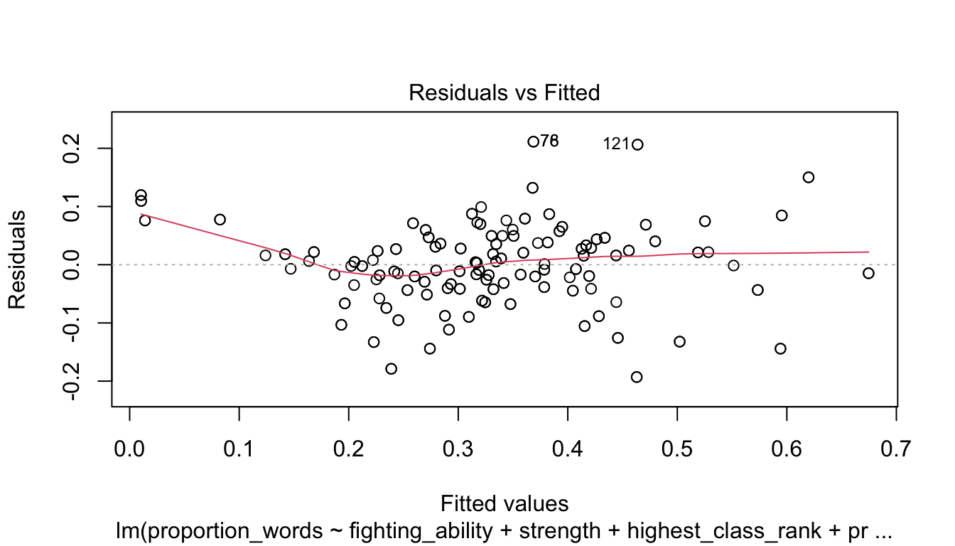
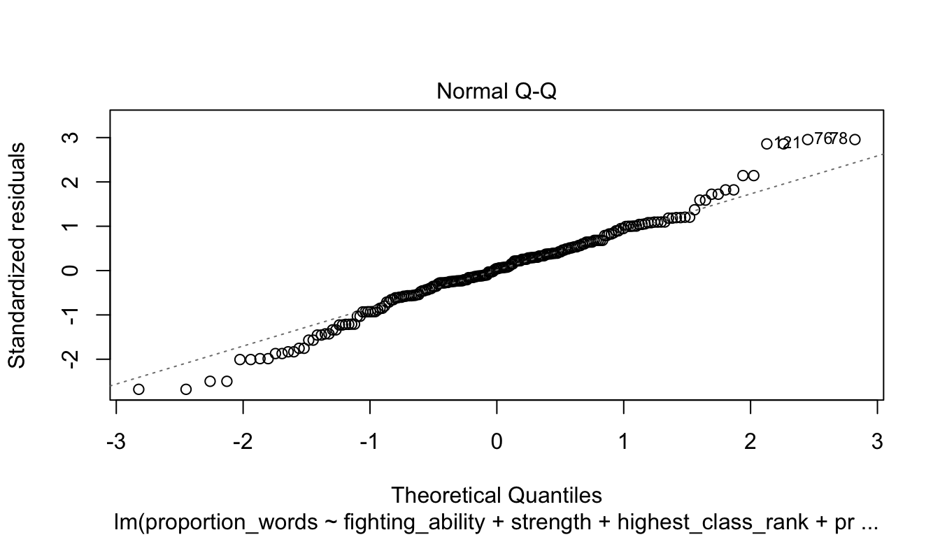
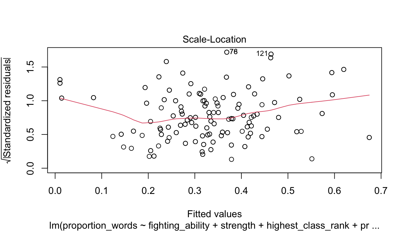
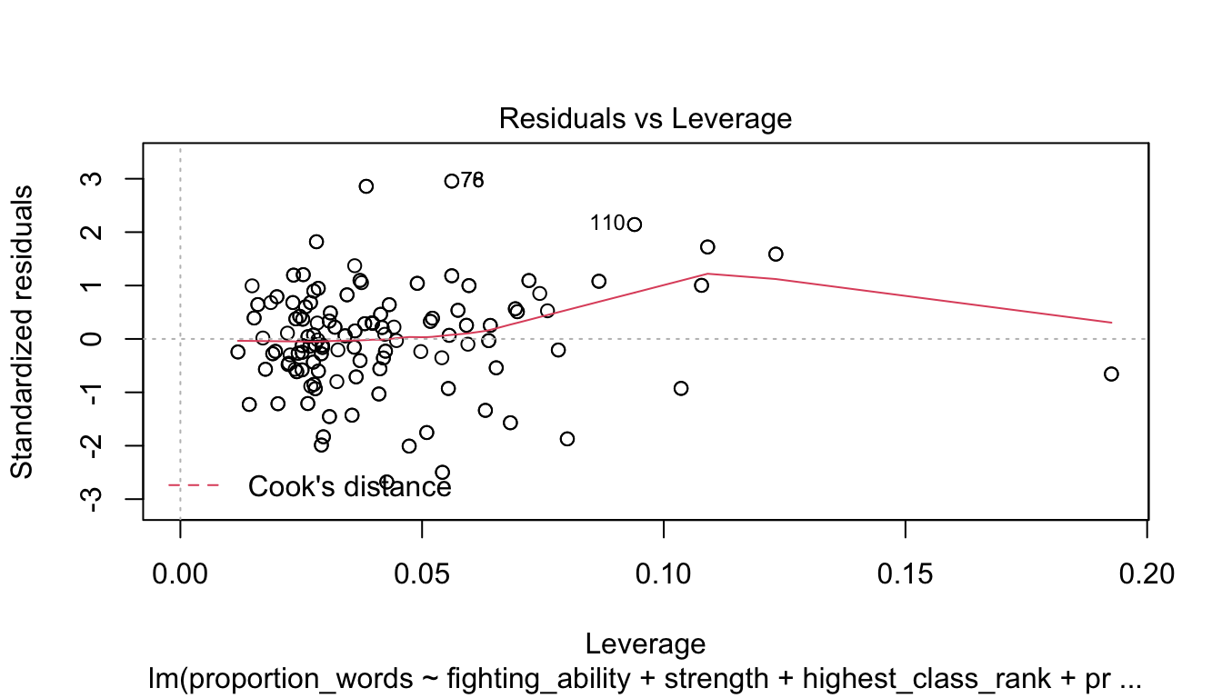
These look pretty good, except that there may be 3-4 values that don’t seem to be following the rest of the trend. See for example the residuals versus fitted plot with the 4 values on the left.
To summarize, here is a method for doing stepwise regression using \(p\)-values.
- Group the variables into variables that naturally belong together, if possible.
- Remove the non-significant variables in a group, checking each time to see whether the significance of other variables has changed. If a variable is categorical, then keep the variable if any of the levels of the variable are significant.
- Use
anovato see whether any of the variables that were removed are significant. If so, test one-by-one to try to find one to put back in the model. - Move to the next group of variables and continue until all of the variables are significant.
Doing stepwise regression like this is not without its detractors. One issue is that the final model is very much dependent on the order in which we proceed. If we had removed f2_psychopathy first, how would that have affected things? Can we justify our decision to remove f1_psychopathy first? Certainly not. The resulting model that we obtained is simply a model for the response. We are not claiming that it is the best one. It is also very possible that the variables that we removed are also good predictors of the response. We should not make the conclusion that the other variables aren’t related.
That being said, stepwise regression for variable selection is quite common in practice, which is why we include it in this book.
The technique we used above was based on \(p\)-values. One can also use other measures of goodness of fit of a model to perform stepwise regression. A common one is the Akaike Information Criterion, which we do not explain here, but we show how to use it to find a parsimonious model. The implementation of this is nice because at each decision point, the algorithm tests what would happen if we add back in any of the variables that we have removed as well as what would happen if we remove any of the variables that we currently have.
##
## Call:
## lm(formula = proportion_words ~ f2_psychopathy + total_psychopathy +
##     fighting_ability + strength + highest_class_rank + dyad_status_difference +
##     proportion_sequence_starts + interruptions_per_min + sequence_starts_per_word_x100 +
##     interruptions_per_word_x100 + affect_words, data = converse)
##
## Residuals:
##       Min        1Q    Median        3Q       Max
## -0.189974 -0.036895  0.000572  0.044182  0.190963
##
## Coefficients:
##                                Estimate Std. Error t value Pr(>|t|)
## (Intercept)                    0.304026   0.020184  15.063  < 2e-16 ***
## f2_psychopathy                -0.013849   0.007641  -1.812 0.071434 .
## total_psychopathy              0.018827   0.007876   2.390 0.017773 *
## fighting_ability              -0.032058   0.008090  -3.963 0.000103 ***
## strength                       0.020196   0.008139   2.481 0.013919 *
## highest_class_rank             0.024566   0.011126   2.208 0.028394 *
## dyad_status_difference        -0.015754   0.006712  -2.347 0.019909 *
## proportion_sequence_starts     0.479287   0.039657  12.086  < 2e-16 ***
## interruptions_per_min          0.106362   0.014115   7.536 1.70e-12 ***
## sequence_starts_per_word_x100 -0.047826   0.005855  -8.168 3.63e-14 ***
## interruptions_per_word_x100   -0.071390   0.009274  -7.698 6.42e-13 ***
## affect_words                  -0.005436   0.002393  -2.272 0.024170 *
## ---
## Signif. codes:  0 '***' 0.001 '**' 0.01 '*' 0.05 '.' 0.1 ' ' 1
##
## Residual standard error: 0.07246 on 198 degrees of freedom
## Multiple R-squared:  0.7472, Adjusted R-squared:  0.7332
## F-statistic: 53.21 on 11 and 198 DF,  p-value: < 2.2e-16
In this case, the AIC derived model includes all of the variables that we included, plus f2_psychopathy, total_psychopathy, and dyad_status_difference. These variables do not all pass the \(p\)-value test, but notice that the adjusted \(R^2\) of the AIC derived model is higher than the adjusted \(R^2\) of the model that we chose. The two models have their pros and cons, and as is often the case, there is not just one final model that could make sense.
Vignette: Data in Other Formats
By this point in the book, we hope that you are comfortable doing many tasks in R. We like to imagine that when someone gives you data in the future, your first thought will be to open it up in R. Unfortunately, not everyone is as civilized as we are, and they may have saved their data in a format that doesn’t interact well with R. This vignette gives some guidance for what to do in that case.
First, as a general recommendation, never make any modifications directly to the data set that you were given. That data should stay in the exact same state, and ideally, you would document every change and decision that you make while getting the data ready to be read into R. In particular, never write over the original data set.
If the data you receive is in comma-separated or tab-separated format (typical extensions are .csv or .tsv), then you can read it in with read.csv(file = "your_file_name.csv"). The default separator is a comma, so if you are reading in a tab separated values file, you will need to add read.csv(file = "your_file_name.tsv", sep = "\t"). If the data is stored with the first row being the variable names, and each subsequent row being data, then this just works. If it doesn’t work correctly, then you may want to open the data up in a spreadsheet and manipulate it there until it is in the easiest format to read.
If the data is .xls or .xlsx, then you will almost always need to open it in Google Sheets or Excel. You might try readxl::read_xls("your_file_name.xls", sheet = 1) or readxl::read_xlsx(your_file_name.xlsx, sheet = 1), but this will typically only work well if the data has been prepared by someone who understands the importance of having rectangular data. Many, if not most, data that is stored in this format has data and metadata stored in the file itself. Often, people will merge cells to indicate something, or they may have 5 rows of headers with various descritpions of the variables. They may have cells at the end that compute the mean and standard deviation of the columns; those aren’t data! We’ve seen any number of things that need to be changed so that the file can be read into R. Unfortunately, this process is not normally reproducible, so you will at a minimum want to hold on to the original data set. We recommend making the changes in a spreadsheet and then saving to a .csv file, which can easily be read into R. If you want your process to be reproducible, there are ways of doing this totally inside of R, but it can be challenging.
If the extension is .RData or .Rda, your file is likely an R Data file, and can be loaded into R via load("file_name.RData"). This is the easiest case to deal with for an R user!
If the extension is .dat (MATLAB), .dta (Stata), .sav (SPSS), .sas7bdat (SAS), then you can use the haven package to load the data into R with, e.g. haven::read_dat(), haven::read_stata(), haven::read_spss() or haven::read_sas(). This usually works well, though the format of the imported data can seem a bit odd. If you run across a data set in a different extension than what has been mentioned here, then you can either convert it to one of the formats listed above, or look for a speciality package that can read your data type into R. Chances are, there is one out there.
Exercises
-
Consider again the
conversationdata set in thefosdatapackage. Suppose that we wanted to model the proportion of words spoken on variables that would be available before the conversation. Find a parsimonious model of the proportion of words spoken ongender,f1_psychopathy,f2_psychopathy,total_psychopathy,attractiveness,fighting_ability,strength,height,median_income,highest_class_rank,major_presigeanddyad_status_difference. -
Consider the data set
cigs_small, which is in thefosdatapackage. The Federal Trade Commission tested 1200 brands of cigarettes in 2000, and reported the carbon monoxide, nicotine, and tar content along with other identifying variables. The data set insmall_cigscontains one randomly selected cigarette from each brand that made a 100 cigarette in 2000. Find a parsimonious model ofcoon the variablesnic,tar,packandmenthol. -
Consider the data set
fish, which is in thefosdatapackage. This data set consists of the weight, species, and 5 other measurements of fish. Find a parsimonious model ofweighton the other variables. Note that there are many missing values forgender. -
Consider the data set
tlcin theISwRpackage. Model the variabletlcinside the data settlcon the other variables. Include plots and examine the residuals. -
Consider the
cystfibrdata set in theISwRpackage. Find a parsimonious linear model of the variablepemaxon the other variables. Be sure to read about the variables so that you can guess which variables might be grouped together. -
Consider the
seoulweatherdata set, which can be read viaread.csv("http://stat.slu.edu/~speegle/_book_data/"Bias_correction_ucl.csv). This data was downloaded here, where you can also read about the variables. We wish to model the error in the next day forecast on the variables that we knew on the present day. (That is, all variables except forNext_TmaxandNext_Tmin.)- Find a parsimonious model of the error on the other variables.
- What percentage of the error in the next day prediction is explained by your model?
-
Load the data set
MRex2.csvfrom http://stat.slu.edu/~speegle/_book_data/MRex2.csv. This data set contains the following variables:- G = The total number of games played in the AL or NL each year.
- HR = The number of home runs hit per game.
- R = The number of runs scored per game.
- SB = The number of stolen bases per game.
- CS = The number of times caught stealing per game.
- IBB = The number of intentional bases on balls per game.
- X2B = The number of doubles hit per game.
- AB = The number of at bats per game.
- PSB = The percentage of time a base stealer was successful.
- yearID = the year in question.
Load the data frame and complete the following tasks:
- Compute the correlation coefficient for each pair of variables. Comment on pairs that are highly correlated.
- Create a scatterplot of Runs scored per game versus each of the other 8 variables.
- Create a linear model of the number of runs scored per game on all of the other variables except
yearID. - CS is considered a bad thing to happen, and leads to fewer runs being scored. Why is the coefficient associated with CS positive?
- Are SB, CS and PSB individually significant?
- Are SB, CS and PSB jointly significant?
- Intelligently remove variables and create a model that describes the response.
- Examine the residuals, and evaluate your model.
-
In this problem, we will use simulation to show that the \(F\) statistic computed by
lmfollows the \(F\) distribution.- Create a data frame where
x1andx2are uniformly distributed on \([-2, 2]\), and \(y = 2 + \epsilon\), where \(\epsilon\) is a standard normal random variable. - Use
lmto create a linear model of \(y = \beta_0 + \beta_1 x_1 + \beta_2 x_2\). - Use
summary(mod)$fstatistic[1]to pull out the \(F\) statistic. - Put inside
replicate, and create 2000 samples of the \(F\) statistic (for different response variables). - Create a histogram of the \(F\) statistic and compare to the pdf of an \(F\) random variable with the correct degrees of freedom. (There should be 2 numerator degrees of freedom and \(N\) - 3 denominator degrees of freedom.)
- Create a data frame where
-
In this problem, we examine robustness to normality in
lm.- Create a data frame of 20 observations where
x1andx2are uniformly distributed on \([-2, 2]\), and \(y = 1 + 2 * x_1 + \epsilon\), where \(\epsilon\) is exponential with rate 1. - Use
lmto create a linear model of \(y = \beta_0 + \beta_1 x_1 + \beta_2 x_2\), and usesummary(mod)$coefficients[3,4]to pull out the \(p\)-value associated with a test of \(H_0: \beta_2 = 0\) versus \(H_a: \beta_2 \not= 0\). - Replicate the above code and estimate the proportion of times that the \(p\)-value is less than .05.
- How far off is the value from what you would expect to get from the theory?
- Create a data frame of 20 observations where