Chapter 1 Posterior Analysis
In this chapter, we learn how to answer questions about our populations (at least probabilistically) based on the sample from the posterior that we obtain. The idea is that the sample from the posterior is our best guess at what the posterior distribution of the parameters is, so we can estimate any1 probability related to the parameters through the sample from the posterior.
This chapter consists entirely of examples, with a little bit of text explaining why we did what we did.
1.1 Credible Interval for the Mean (Normal-Normal)
Consider the plastics data set in the fosdata package. Construct a 95 percent credible interval for the mean diameter of the plastics.
We start by loading the data into R and removing the missing values for diameter.
library(tidyverse)
library(rstan)
library(bayesplot)

plastics <- fosdata::plastics
b1 <- plastics %>%
  filter(!is.na(diameter))
Let’s look at a histogram of the diameters.
hist(b1$diameter)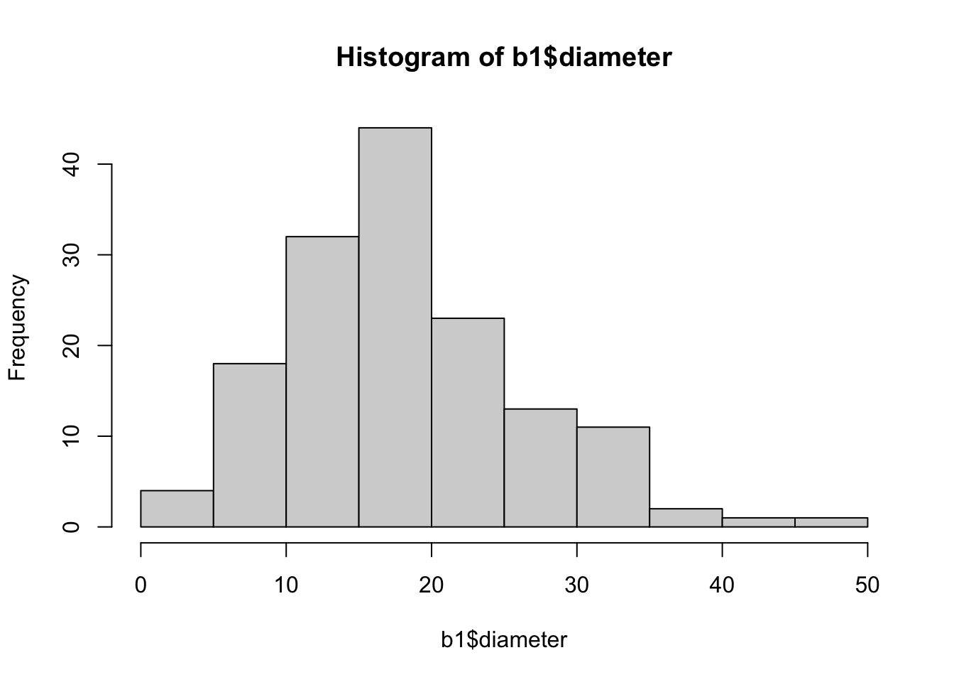
The diameters are right-skewed, but we ignore that and model them via a normal random variable anyway. If we wanted to get the best possible model for diameters of plastics, then we would need to modify this.
Here is the model that we use:
data {
  int n;
  real y[n];
}
parameters {
  real<lower = 0> sigma;
  real mu;
}
model {
  y ~ normal(mu, sigma);
  mu ~ normal(0, 1000);
  sigma ~ uniform(1.0/100.0, 1000);
}
You can download this file and store in a file called normal.stan if you want it on your computer.
Let’s go through the model line by line, since we don’t have notes from that chapter typed up. The data block lists all of the data that we will be passing from R to the model. In this case, we are passing n, the number of samples in the data, and y, the observed diameters of the plastics.
When we pass the data from R to stan, we need to make sure we use exactly the same names! Including capitalization!
data {
  int n;
  real y[n];
}
Next, we have the parameters of the model. These go hand-in-hand with the model itself below; you can’t know what goes in one block without knowing what goes in the other block. In this case, since we are modeling the diameters as normal with unknown mean and standard deviation, we have two parameters: mu which can be any real number and sigma which must be a positive real number.
parameters {
  real<lower = 0> sigma;
  real mu;
}
Finally, we have the model itself. We need to include the model for the data (diameters of plastics, but not n because that isn’t random, or at least we aren’t modeling the randomness associated with it). We are modeling the data as normally distributed in the first line, with unknown mean and standard deviation. In the second line, we are giving a prior for the mean. We are trying to give a vague prior, and since all of the values of the diameters are between 0 and 50, setting the sd to 1000 and mean to 0 in the prior seems vague. In the third line, we are setting a vague prior for sigma. Again, since the true value is likely around 10, uniform between .01 and 1000 is vague.
model {
  y ~ normal(mu, sigma);
  mu ~ normal(0, 1000);
  sigma ~ uniform(1.0/100.0, 1000);
}Do not write 1/100 inside of code like this, as it will get truncated to 0. Use 1.0/100.0 to indicate you want a real number answer to the proble, 1/100.
bayes_model <- stan(
  "stan_models/normal.stan",
  data = list(
    y = b1$diameter,
    n = nrow(b1)
  ),
  chains = 4, # this is the default, we don't need it
  iter = 5000 * 2,
  seed = 4880,
  refresh = 0 # eliminates some of the output so that it runs quietly
)
After building our model, we want to be able to examine the samples from the model. We pull those out as follows:
sim_data <- as.array(bayes_model, pars = c("mu", "sigma"))Now, we do some diagnostic plots to see whether the simulations have converged, and to assess the simulations in other ways. Again, since we don’t have notes up from the previous chapters, I go over each diagnostic briefly:
mcmc_acf(sim_data)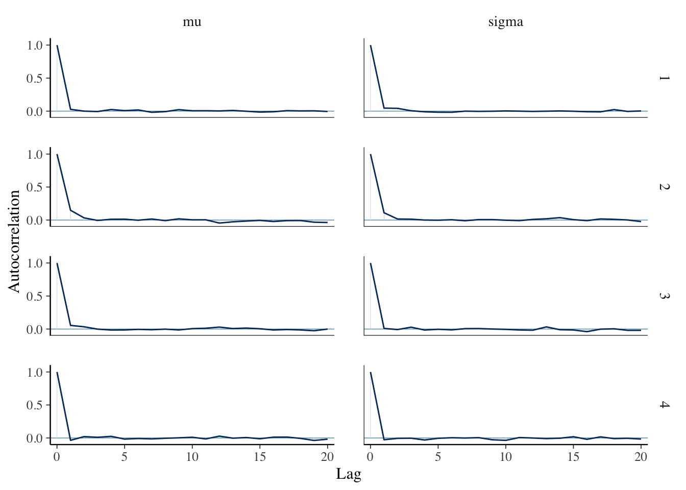
This looks fine. There is some autocorrelation, but not an excessive amount. Remember, it is bad if the acf stays high for a long period of time, or if the acf looks drastically different in the different chains.
coda::effectiveSize(sim_data[, , "mu"])## chain:1 chain:2 chain:3 chain:4
## 4735.177 3704.902 4208.499 5365.151coda::effectiveSize(sim_data[, , "sigma"])## chain:1 chain:2 chain:3 chain:4
## 4213.584 4001.540 5000.000 5271.515These go with the correlogram above. We expect them to be fine, which they are. The true sample sizes are 5000, and the effective sizes are close to that. The book recommends an effective sample size of at least 10 percent of the true size as a rule of thumb.
mcmc_dens_chains(sim_data)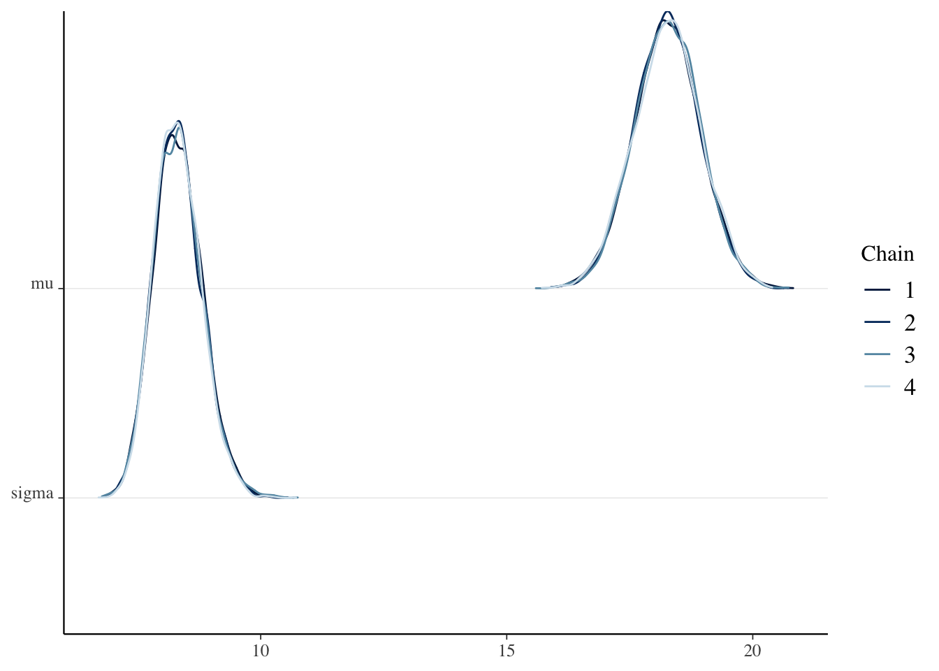
The four chains seem to have converged to the same distribution for sigma and for mu.
Rhat(sim_data[, , "mu"])## [1] 1.000044Rhat(sim_data[, , "sigma"])## [1] 1.000059Another diagnostic testing to see whether the chains have converged to the same distribution. The book recommends \(\hat R < 1.05\) as a rule of thumb.
mcmc_trace(sim_data)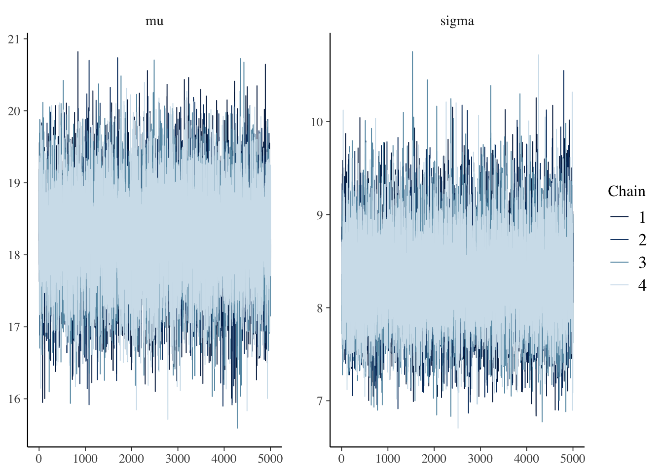
Trace plots. The chains seem to be the same, and they seem to be well-mixing. Recall that we don’t want the chain to spend a large percentage of its time in one part of the distribution and then switch to the other part of the distribution. That would not be well-mixing.
Taken as a group, the diagnostics indicate that we are good to continue.
To compute the 95 percent credible interval, we use hdi:
HDInterval::hdi(sim_data[, , "mu"])## chains
## chain:1 chain:2 chain:3 chain:4
## lower 16.94223 16.9104 16.90980 16.93453
## upper 19.67868 19.5291 19.53861 19.60543
## attr(,"credMass")
## [1] 0.95All four chains give similar answers, which is good. For a final answer we can combine all of the chains into a single sample as follows:
HDInterval::hdi(as.vector(sim_data[, , "mu"]))## lower upper
## 16.94010 19.60956
## attr(,"credMass")
## [1] 0.95A 95 percent credible interval for mu, the mean diameter of plastics found in ice floes, is \([16.9, 19.6]\).
- Re-do the entire above analysis and confirm that there is not much change in the credible interval after changing the priors as below:
model {
  y ~ normal(mu, sigma);
  mu ~ normal(0, 100);
  sigma ~ uniform(1.0/10.0, 100);
}- What if you changed your priors to
mu ~ normal(0, 1)andsigma ~ uniform(1, 5)? Which diagnostic(s) would have led you to realize that your model is not working?
1.2 Credible interval for the mean (Gamma-Poisson)
We do a similar analysis as in Section 1.1, but this time the data we have is Poisson. Consider the 2015 World Cup, and we analyze the total number of scores.
ww <- fosdata::world_cup %>%
  filter(str_detect(competition, "2015"))
plot(table(ww$score_1 + ww$score_2))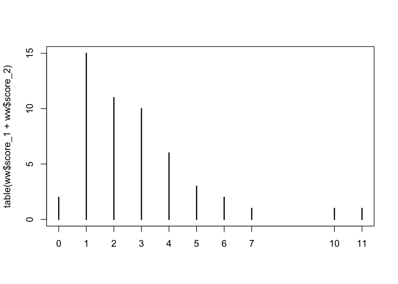
The stan model we need is given below, where we choose a vague prior for lambda, the mean of the Poisson distrubution.
data {
  int n;
  int<lower = 0> y[n];
}
parameters {
  real<lower = 0> lambda;
}
model {
  y ~ poisson(lambda);
  lambda ~ gamma(0.1, 0.1);
}
You can download this file and use it to run the following code.
bayes_model <- stan(
  "stan_models/gamma_poisson.stan",
  data = list(
    y = c(ww$score_1, ww$score_2),
    n = 2 * nrow(ww)
  ),
  iter = 5000 * 2,
  seed = 4880,
  refresh = 0 # eliminates some of the output so that it runs quietly
)
sim_data <- as.array(bayes_model, pars = "lambda")We run a few diagnostics to check convergence.
mcmc_acf(sim_data)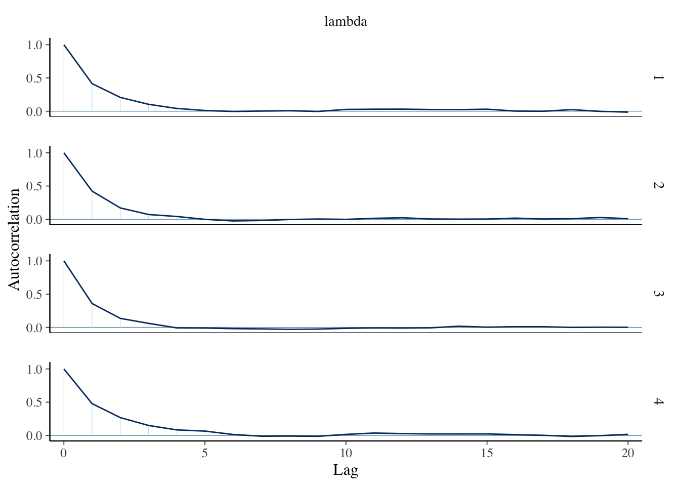
mcmc_dens_chains(sim_data)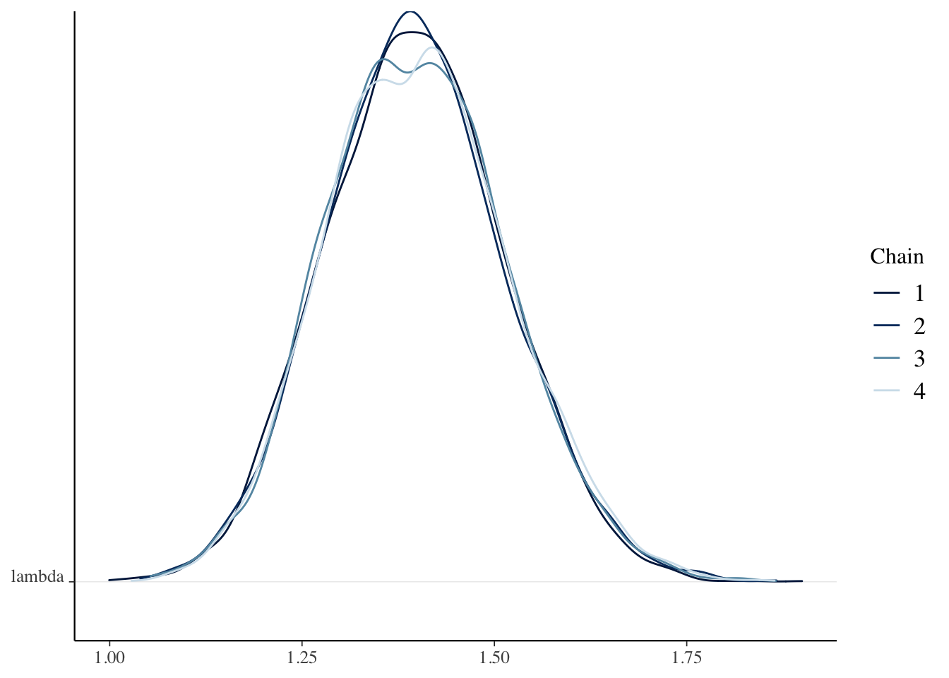
Rhat(sim_data[, , "lambda"])## [1] 1.000631And now we can get a 95 percent credible interval for the rate at which goals are scored:
HDInterval::hdi(sim_data)## lower upper
## 1.173088 1.629433
## attr(,"credMass")
## [1] 0.95We conclude that a 95 percent credible interval for the rate at which goals are scored is \([1.17, 1.63]\).
1.3 ROPEs and Difference of Means
In this section, we discuss Bayesian hypothesis testing. We consider the data from fosdata::normtemp, which gives the temperature of healthy adults. Our null hypothesis is:
\(H_0: \mu = 98.6\) versus \(H_a: \mu\not= 98.6\).
Following Kruschke, we define a region of practical equivalence (ROPE), which indicates a range of values for which a departure from the null hypothesis would not have a practical effect. In the context of body temperature, if the mean body temperature of healthy adults turns out to be 98.5, would that have a clinical significance? Possibly not. We might want to check with experts to find out, though. In this case, imagine that we talk to experts and decide that a mean temperature between 98 and 99.2 would not have any practical effect, so we define the ROPE to be \([98, 99.2]\).
Our plan is to compute a credible interval and then see how it compares to the ROPE. There are three possibilities:
1. The credible interval is completely inside of the ROPE. This **confirms** the null hypothesis.
2. The credible interval is completely outside of the ROPE. We reject the null hypothesis in favor of the alternative.
3. The credible interval has pieces both inside and outside of the ROPE. The test is inconclusive, and we would need more data to make a decision.
Let’s load the data and see how to do it in this specific instance.
nn <- fosdata::normtemp
hist(nn$temp)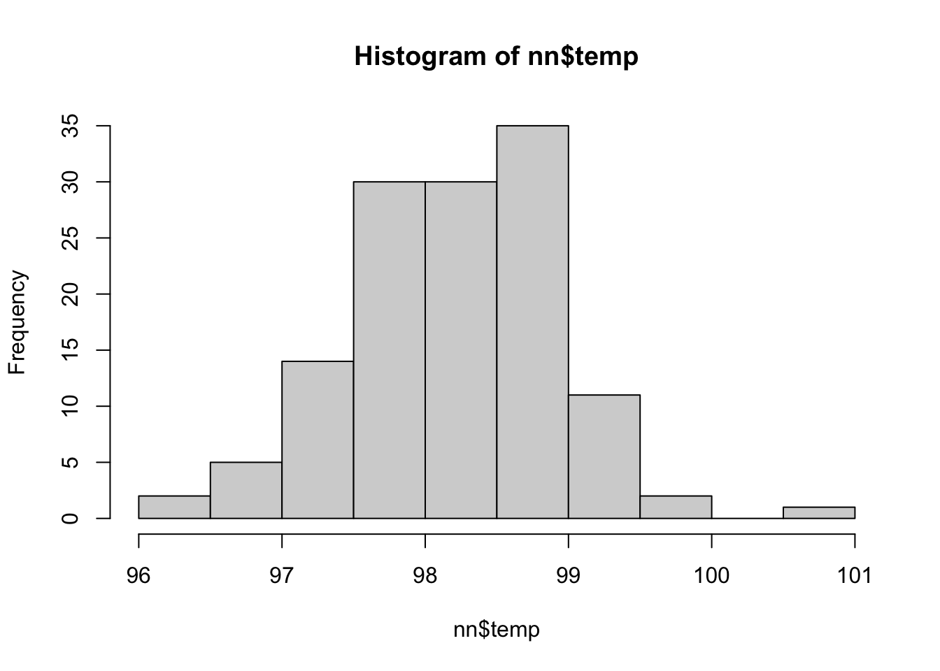
We can use the same model as the one we used above:
data {
  int n;
  real y[n];
}
parameters {
  real<lower = 0> sigma;
  real mu;
}
model {
  y ~ normal(mu, sigma);
  mu ~ normal(0, 1000);
  sigma ~ uniform(1.0/100.0, 1000);
}
Note that a prior on mu of normal(0, 1000) still appears to be a vague prior.
bayes_model <- stan(
  "stan_models/normal.stan",
  data = list(
    y = nn$temp,
    n = nrow(nn)
  ),
  iter = 5000 * 2,
  seed = 4880,
  refresh = 0 # eliminates some of the output so that it runs quietly
)
We run a couple of different diagnostics:
mcmc_trace(bayes_model, pars = c("sigma", "mu"))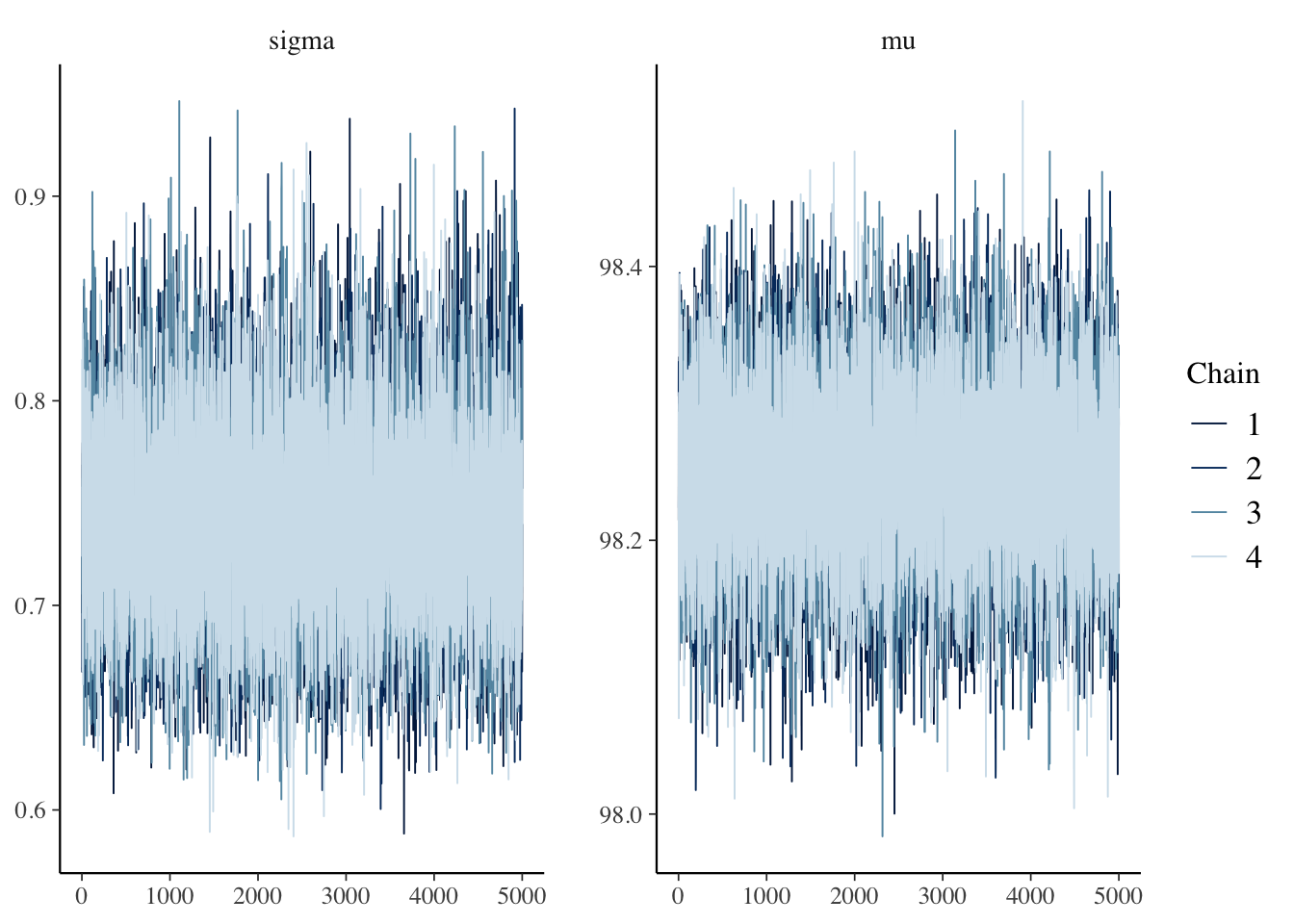
sim_data <- as.array(bayes_model, pars = c("sigma", "mu"))

Rhat(sim_data[, , "mu"])
## [1] 1.000097Rhat(sim_data[, , "sigma"])## [1] 1.000084mcmc_dens_chains(sim_data, pars = "mu")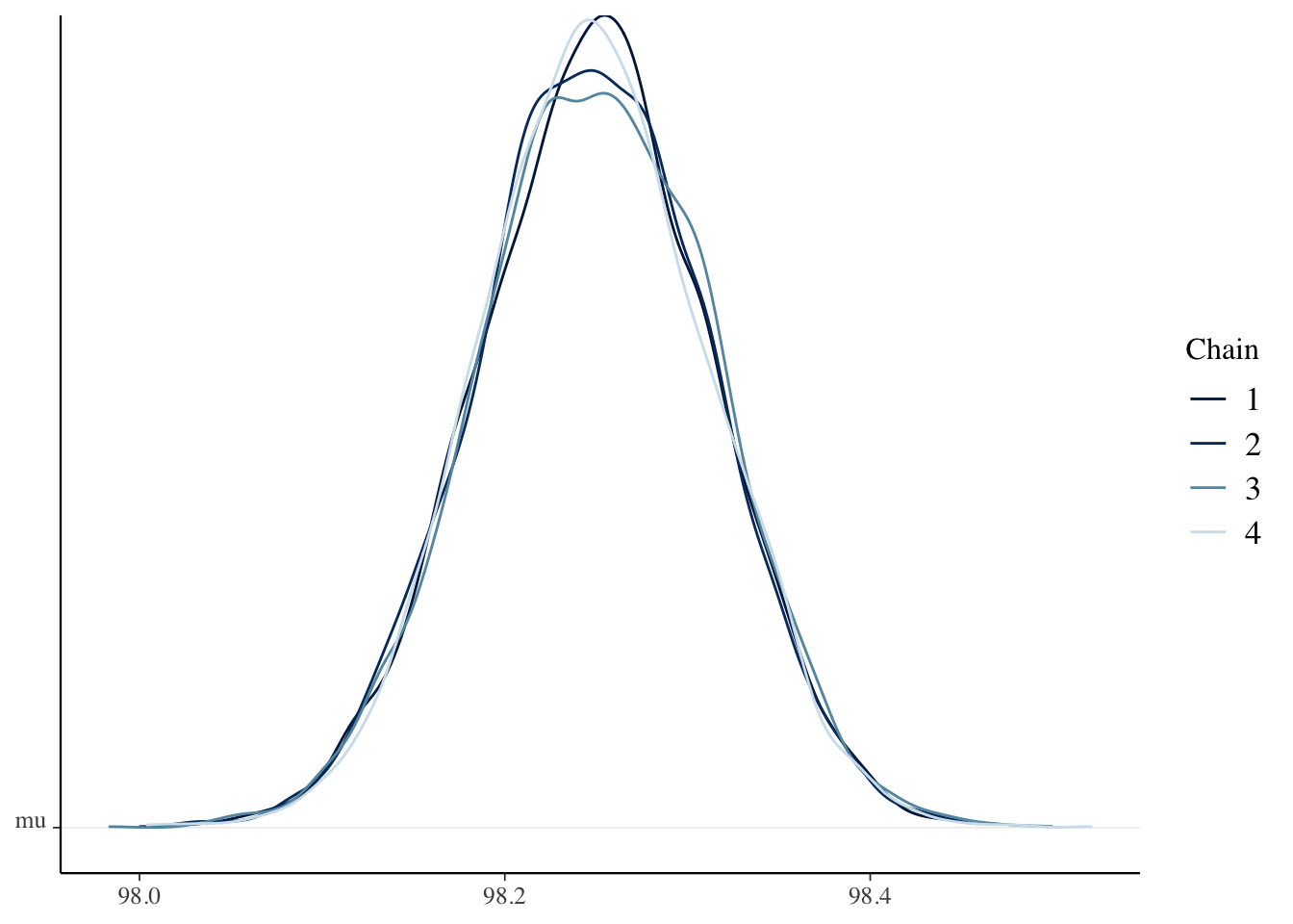
coda::effectiveSize(sim_data[, , "mu"])## chain:1 chain:2 chain:3 chain:4
## 4016.946 4197.318 5000.000 4630.540Things look pretty good, so we compute a credible interval.
HDInterval::hdi(sim_data[, , "mu"])## chains
## chain:1 chain:2 chain:3 chain:4
## lower 98.11437 98.12488 98.12329 98.12478
## upper 98.36370 98.37382 98.37403 98.36682
## attr(,"credMass")
## [1] 0.95The chains all seem to agree on what the credile interval is, so let’s combine the chains and find a final answer for the credible interval:
HDInterval::hdi(as.vector(sim_data[, , "mu"]))## lower upper
## 98.12485 98.37331
## attr(,"credMass")
## [1] 0.95The credible interval is \([98.1, 98.4]\), which is completely contained inside of the ROPE, \([98, 99.2]\). The null hypothesis is confirmed. Note that this is very different than what happens when you do not use a ROPE. In those cases, it is impossible to confirm the null hypothesis, you simply fail to reject it.
Let’s look at an example where we examine the difference in two proportions. Let’s look at the coin tossing data we discussed in class found here, and we see whether there is a difference between the first two coin tossers.
Each person tossed 300 times. The first person got 162 H/138 T and the second person got 175 H and 125 T. In this case, we will want our ROPE to be very small, because any real difference in ability to toss heads is interesting. Se set the ROPE of the difference in proportions to be \([-0.005, 0.005]\). Our model looks like this:
data {
  int n;
  int y1;
  int y2;
}
parameters {
  real<lower = 0, upper = 1> pi1;
  real<lower = 0, upper = 1> pi2;
}
model {
  y1 ~ binomial(n, pi1);
  y2 ~ binomial(n, pi2);
  pi1 ~ beta(1, 1);
  pi2 ~ beta(1,1);
}
You can download it here.
bayes_model <- stan(
  "stan_models/beta_binomial_2.stan",
  data = list(
    y1 = 162,
    y2 = 175,
    n = 300
  ),
  iter = 5000 * 2,
  seed = 4880,
  refresh = 0 # eliminates some of the output so that it runs quietly
)Check that the diagnostics are OK by doing a trace plot, density plot, acf, R-hat and effective sample sizes.
sim_data <- as.array(bayes_model)Let’s compute the credible interval of the difference in proportions. We first need to see how to create a sample of differences of proportions. If we subtract the samples from pi2 from the samples from pi1, we get a sample of the differences. Here are the first 6 rows of the resulting matrix. We see that the results are more often negative than postive, but they are also sometimes positive.
head(sim_data[, , "pi1"] - sim_data[, , "pi2"])## chains
## iterations chain:1 chain:2 chain:3 chain:4
## [1,] 0.02845320 -0.03010909 -0.046758394 0.01120933
## [2,] -0.03057890 -0.02425073 -0.020945915 -0.10461946
## [3,] -0.04589529 -0.05252479 -0.051746370 0.07351009
## [4,] -0.06939679 -0.07522395 -0.004354386 0.04327570
## [5,] -0.01727833 -0.01039030 0.007237696 -0.02779436
## [6,] -0.05998574 -0.10476288 -0.084194296 -0.14470688We use the differences to compute the credible interval.
HDInterval::hdi(sim_data[, , "pi1"] - sim_data[, , "pi2"])## chains
## chain:1 chain:2 chain:3 chain:4
## lower -0.12256826 -0.12411839 -0.11715708 -0.12216112
## upper 0.03237868 0.03489326 0.03445214 0.03712623
## attr(,"credMass")
## [1] 0.95The chains seem to agree on the credible interval for the differences, and we compute the final estimate for the CI of \(p_2 - p_1\):
HDInterval::hdi(as.vector(sim_data[, , "pi1"] - sim_data[, , "pi2"]))## lower upper
## -0.12216373 0.03445794
## attr(,"credMass")
## [1] 0.95Our CI is \([-.122, .034]\), which has pieces both inside and outside the ROPE, so the test is inconclusive. The participants may or may not have the same probability of tossing heads.
1.4 Sampling from the posterior
Let’s return to our original plastics example, where we have a single variable diameter that we are modeling as normal with unknown mean and standard deviation. We can estimate probabilities associated with future observations by creating samples following the posterior distribution of \(\mu\) and \(\sigma\). I assume that you have re-run the following code to get your posterior samples from mu and sigma.
plastics <- fosdata::plastics
b1 <- plastics %>%
  filter(!is.na(diameter))

bayes_model <- stan(
  "stan_models/normal.stan",
  data = list(
    y = b1$diameter,
    n = nrow(b1)
  ),
  chains = 4,
  iter = 5000 * 2,
  seed = 4880,
  refresh = 0
)

sim_data <- as.array(bayes_model, pars = c("mu", "sigma"))
Let’s turn this array into two vectors. The first vector is going to have all of the samples from the mean:
all_mu <- as.vector(sim_data[, , "mu"])and the second vector is going to have all of the samples from the standard deviation:
all_sigma <- as.vector(sim_data[, , "sigma"])Check that all_mu[1] is the top left entry in sim_data[,,"mu"]. Which entry in all_mu is the first entry in the second column?
Recall that there are 5000 samples in each chain.
We note that the means and the standard deviations are paired, in the sense that it wouldn’t be correct to associate all_mu[1] with all_sigma[2]. We must associate all_mu[1] with all_sigma[1]. So, if we wanted to simulate a single random sample from the population we have modeled, we could use:
rnorm(1, all_mu[1], all_sigma[1])## [1] 17.86345To get a sample of size 5, we could use:
rnorm(5, all_mu[5], all_sigma[5])## [1] 32.55202 19.47879 16.14033 25.95052 23.13309If we have modeled the data well, then these values should be representative of future diameters of plastics that we might observe, and we can use that information to answer questions.
For example, what is the probability that a piece of plastic has diameter greater than 35? We start by taking a random sample of size 20000 (which is all of the info that we have)
plastic_sample <- rnorm(20000, all_mu, all_sigma)We then compute the percentage of samples that are bigger than 35:
mean(plastic_sample > 35)## [1] 0.02355We see the probability is a little bit more than 2 percent. This doesn’t quite match the observed percentage of plastics which have diameters larger than 35, but it is a prediction of future behavior based on our model.
Create a density plot of future samples of plastic diameters based on your model.
To create a density plot, we take our large sample and use the following command:
plot(density(plastic_sample))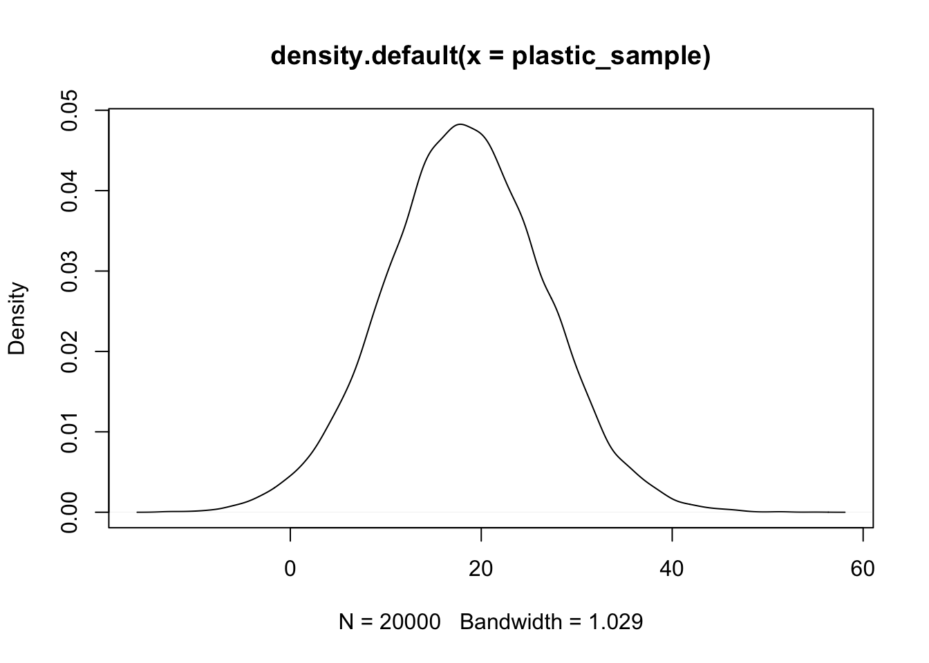
We can also use this is a diagnostic if we compare this density to the historgram of true values that we observed. We don’t want a huge difference in these two plots, because that would mean that we have mis-modeled our data.
hist(b1$diameter, probability = T)
lines(density(plastic_sample))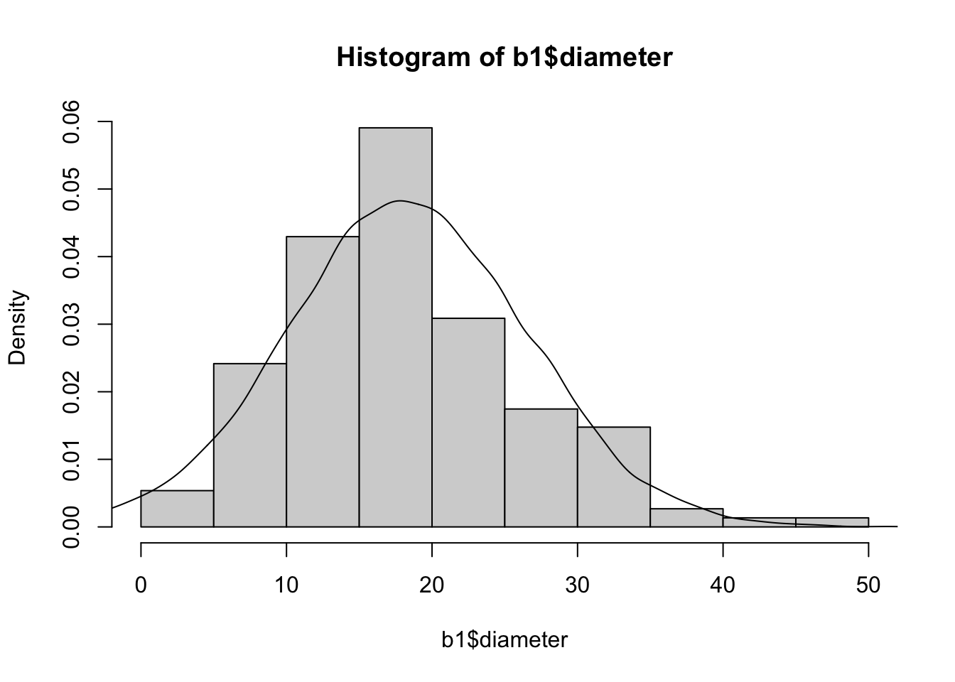
Re-do the diagnostic in the example above using a prior of mu ~ normal(0, 1) and sigma ~ uniform(1, 5) to see what a very poor fit looks like. That is an extreme example, which would definitely indicate a re-thinking of the model is necessary.
Exercises
Well, maybe not any question.↩︎