Chapter 8 Normal Hierarchical Models with No Predictors
We follow the material in Chapter 16 pretty closely. Let’s consider the spotify data set in the bayesrules package.
spotify <- bayesrules::spotify
spotify
## # A tibble: 350 × 23
## track_id title artist popularity album_id album_name album_release_d…
## <chr> <chr> <fct> <dbl> <chr> <chr> <chr>
## 1 7sYAS4C… On &… Alok 79 2a9AGiv… On & On 2019-11-22
## 2 1YSwQvw… All … Alok 56 2FdyKqN… All The L… 2019-07-19
## 3 39cmB3Z… Hear… Alok 75 6fpsA5a… Hear Me N… 2016
## 4 2Dnb6yP… The … Alok 65 0hH9tb1… The Wall 2019-06-28
## 5 1a5Yu5L… Hear… Alok 52 6apmeAA… Hear Me N… 2016-01-01
## 6 74RrMiu… Toda… Alok 45 3GQZqxm… Toda La N… 2018-05-25
## 7 7sYAS4C… On &… Alok 79 2a9AGiv… On & On 2019-11-22
## 8 0Qp1IH1… The … Alok 61 4w68G9o… The Wall 2019-06-28
## 9 36C0Gw2… Tell… Alok 61 1R2C7EG… Tell Me W… 2019-08-30
## 10 1UTXQrm… Meta… Alok 61 2ds371e… Metaphor 2019-02-01
## # … with 340 more rows, and 16 more variables: playlist_name <chr>,
## # playlist_id <chr>, genre <chr>, subgenre <chr>, danceability <dbl>,
## # energy <dbl>, key <dbl>, loudness <dbl>, mode <dbl>,
## # speechiness <dbl>, acousticness <dbl>, instrumentalness <dbl>,
## # liveness <dbl>, valence <dbl>, tempo <dbl>, duration_ms <dbl>summary(spotify)## track_id title artist
## Length:350 Length:350 Frank Ocean : 40
## Class :character Class :character Camila Cabello: 38
## Mode :character Mode :character Kendrick Lamar: 31
## Beyoncé : 25
## Alok : 19
## TV Noise : 14
## (Other) :183
## popularity album_id album_name
## Min. : 7.00 Length:350 Length:350
## 1st Qu.:45.25 Class :character Class :character
## Median :62.50 Mode :character Mode :character
## Mean :58.40
## 3rd Qu.:73.00
## Max. :94.00
##
## album_release_date playlist_name playlist_id
## Length:350 Length:350 Length:350
## Class :character Class :character Class :character
## Mode :character Mode :character Mode :character
##
##
##
##
## genre subgenre danceability energy
## Length:350 Length:350 Min. :24.00 Min. : 9.24
## Class :character Class :character 1st Qu.:56.40 1st Qu.:50.30
## Mode :character Mode :character Median :68.20 Median :64.60
## Mean :66.04 Mean :63.53
## 3rd Qu.:75.90 3rd Qu.:77.60
## Max. :95.10 Max. :98.20
##
## key loudness mode speechiness
## Min. : 0.000 Min. :-20.700 Min. :0.0000 Min. : 2.54
## 1st Qu.: 1.000 1st Qu.: -8.492 1st Qu.:0.0000 1st Qu.: 4.31
## Median : 6.000 Median : -6.388 Median :1.0000 Median : 7.38
## Mean : 5.286 Mean : -6.987 Mean :0.5543 Mean :11.26
## 3rd Qu.: 9.000 3rd Qu.: -4.960 3rd Qu.:1.0000 3rd Qu.:12.68
## Max. :11.000 Max. : -0.247 Max. :1.0000 Max. :48.50
##
## acousticness instrumentalness liveness valence
## Min. : 0.00178 Min. : 0.00000 Min. : 2.640 Min. : 4.98
## 1st Qu.: 1.25750 1st Qu.: 0.00000 1st Qu.: 9.262 1st Qu.:32.02
## Median : 7.11500 Median : 0.00356 Median :12.900 Median :46.30
## Mean :20.60655 Mean : 7.27060 Mean :18.849 Mean :48.20
## 3rd Qu.:30.95000 3rd Qu.: 0.28200 3rd Qu.:25.475 3rd Qu.:65.20
## Max. :98.30000 Max. :94.10000 Max. :88.900 Max. :95.70
##
## tempo duration_ms
## Min. : 64.92 Min. : 66786
## 1st Qu.:102.00 1st Qu.:179594
## Median :122.96 Median :210292
## Mean :121.47 Mean :215335
## 3rd Qu.:135.18 3rd Qu.:239600
## Max. :207.97 Max. :425123
## This is a collection of information on 350 songs which are on Spotify. In this section, we are going to see how to model the popularity of the songs with no predictors. However, we are going to consider the effect of artist. Let’s start by re-ordering the factor artist to be in terms of decreasing mean popularity.
spotify <- spotify %>%
  select(artist, title, popularity) %>%
  mutate(artist = forcats::fct_reorder(.f = artist, -popularity, .fun = mean))
The sample of spotify songs consists of 44 artists; let’s do a barplot of the number of songs for the artists.
spotify %>%
  count(artist) %>%
  ggplot(aes(x = n)) +
  geom_bar()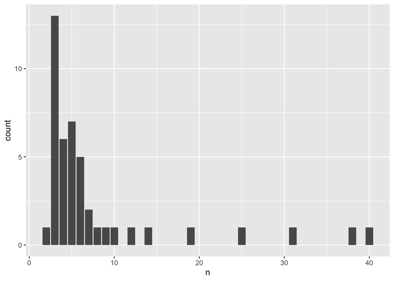
spotify %>%
  group_by(artist) %>%
  summarize(
    mu = mean(popularity),
    n = n()
  )
## # A tibble: 44 × 3
## artist mu n
## <fct> <dbl> <int>
## 1 Camilo 81 9
## 2 Lil Skies 79.3 3
## 3 Camila Cabello 77.1 38
## 4 J. Cole 76.7 12
## 5 Sean Kingston 73 2
## 6 Frank Ocean 69.8 40
## 7 Beyoncé 69.7 25
## 8 Sufjan Stevens 65.7 3
## 9 León Larregui 65.3 3
## 10 Alok 64.8 19
## # … with 34 more rowsEach artist has at least 2 songs, 3 is the most common number of songs, and there are as many as 40 songs for an artist. We have three choices for how to model this, as was described in the previous chapter.
- Complete pooling. We could ignore all of the artist information and put all of the popularities in one bin.
- No pooling. We could separately analyze each artist, with only the common standard deviation of popularity for each artist.
- Partial pooling We could model the data via a hierarchical model. We assume there is a parent distribution of possible means of popularity that artists could have, and that the artists we have are sampled from that parent distribution. We assume that the distribution of popularities of songs for a given artist depends only on the mean of the artist and a standard deviation which is common to all of the artists.
As you can imagine, the first two options will turn out not to be great choices.
8.1 Complete pooled model
We start by setting some notation. Let \(n_j\) be the number of songs that the \(j\)th artist has in the list. Let \(Y_{ij}\) denote the popularity of the \(i\)th song for the \(j\)th artist. So, the list of all samples would look something like
\[ \left((Y_{11}, Y_{21}, \ldots, Y_{n_1 1}), (Y_{12}, \ldots, Y_{n_2 2}) \right) \]
We could look at a density plot of the pooled data, which would give us one model of the outcome.
ggplot(spotify, aes(x = popularity)) +
  geom_density()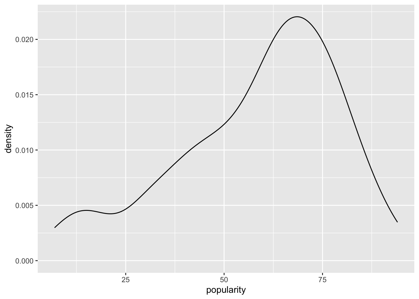
Formally, we could create the following Bayesian model, where the second and third lines are the priors which are obtained via prior_summary in the R chunk below.
- \(Y|_{\mu, \sigma} \sim N(\mu, \sigma)\)
- \(\mu \sim N(50, \mathrm{sd} = 52)\)
- \(\sigma ~ \mathrm{Exp}(0.048)\).
library(rstanarm)
pooled_model <- stan_glm(popularity ~ 1,
  data = spotify,
  prior_intercept = normal(50, 2.5, autoscale = T),
  prior_aux = exponential(1, autoscale = T),
  refresh = FALSE
)
prior_summary(pooled_model)
## Priors for model 'pooled_model'
## ------
## Intercept (after predictors centered)
## Specified prior:
## ~ normal(location = 50, scale = 2.5)
## Adjusted prior:
## ~ normal(location = 50, scale = 52)
##
## Auxiliary (sigma)
## Specified prior:
## ~ exponential(rate = 1)
## Adjusted prior:
## ~ exponential(rate = 0.048)
## ------
## See help('prior_summary.stanreg') for more detailsposterior_vs_prior(pooled_model, group_by_parameter = T, facet_args = list(scales = "free_y"))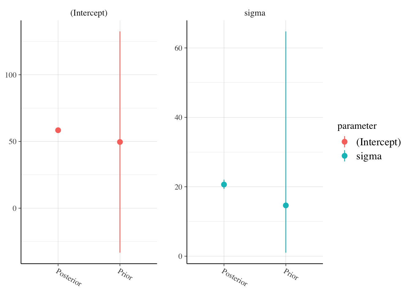
broom.mixed::tidy(pooled_model,
  conf.int = T,
  effects = c("fixed", "aux")
)
## # A tibble: 3 × 5
## term estimate std.error conf.low conf.high
## <chr> <dbl> <dbl> <dbl> <dbl>
## 1 (Intercept) 58.4 1.14 56.6 60.2
## 2 sigma 20.6 0.800 19.4 22.0
## 3 mean_PPD 58.4 1.58 55.8 61.0Based on this model, the popularity of a song is normally distributed with mean about 58.4 and standard deviation about 20.7. Note that this would be true whichever artist we have a song from. This may have been reasonable if we didn’t know anything more about the songs, but is unreasonable given that we know the artist and much more information about the songs.
artist_means <- spotify %>%
  group_by(artist) %>%
  summarize(
    popularity = mean(popularity),
    n = n()
  )

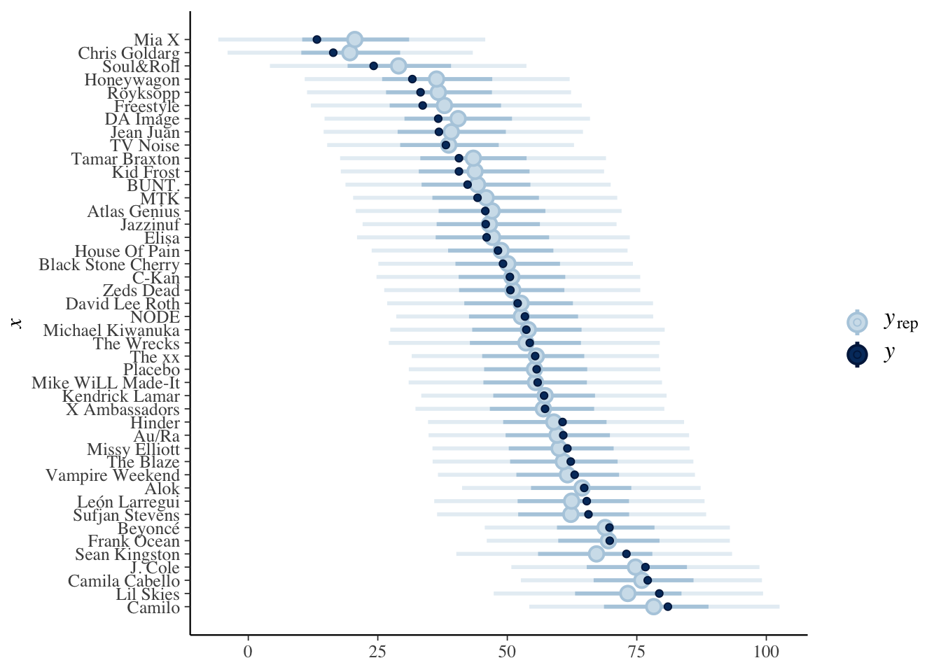
predictions_complete <- posterior_predict(pooled_model, newdata = artist_means)

bayesplot::ppc_intervals(artist_means$popularity, yrep = predictions_complete) +
  scale_x_continuous(
    labels = artist_means$artist,
    breaks = 1:nrow(artist_means)
  ) +
  coord_flip()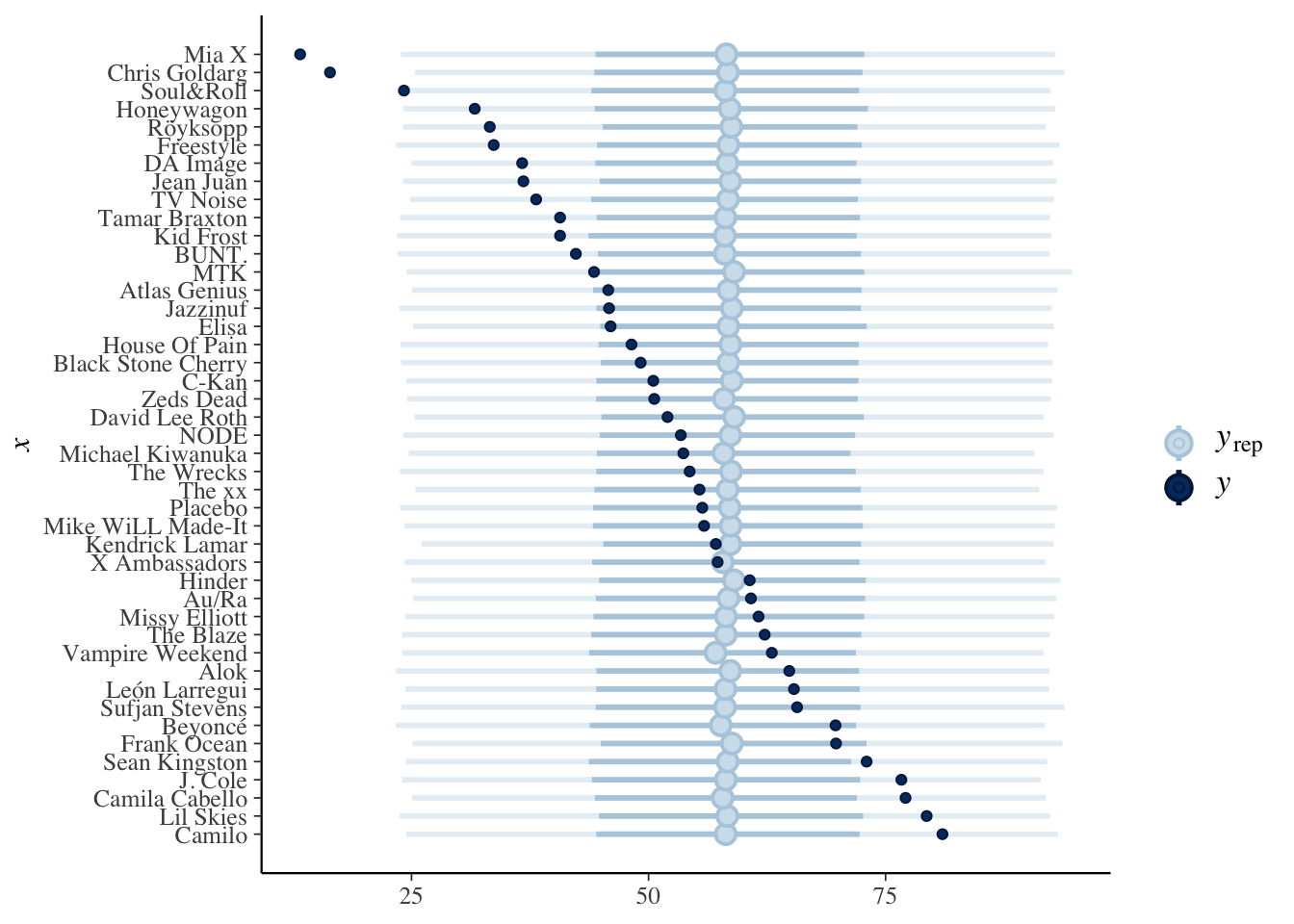
8.2 No pooled model
In this model, we create a separate mean for each artist in our sample. Notationally, we let \(\mu_j\) be the mean popularity of artist \(j\). Here is a plot that sort of illustrates it, but we are not assuming in the below plot that we are estimating the density via a normal distribution with different means and common standard deviation.
ggplot(spotify, aes(x = popularity, color = artist)) +
  geom_density() +
  gghighlight::gghighlight(artist == "Lil Skies" | artist == "Frank Ocean" | artist == "Mia X")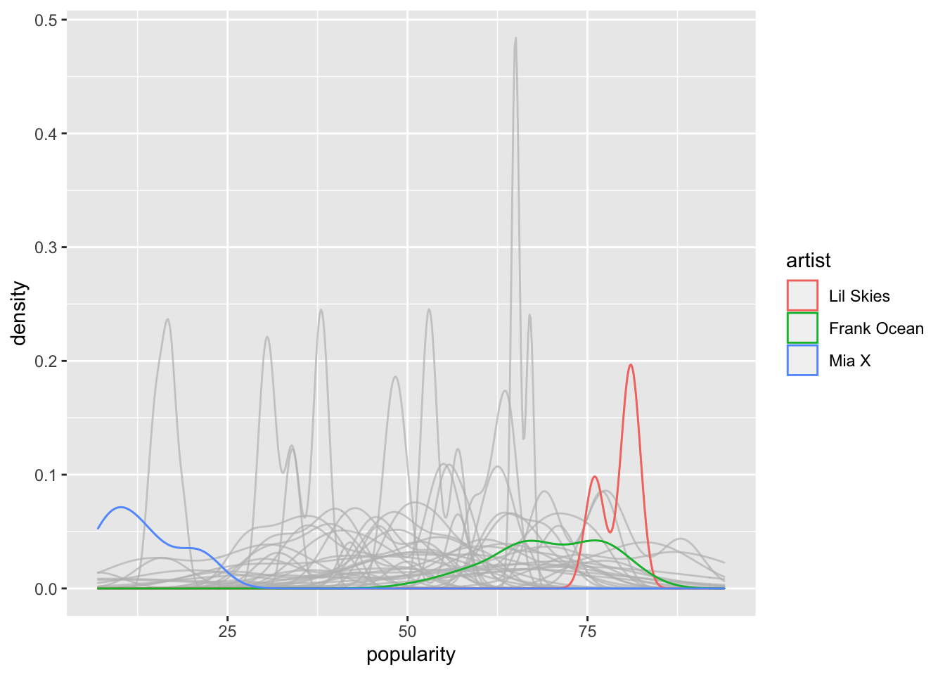
Our model is
- \(Y|_{\mu_j, \sigma} \sim N(\mu_j, \sigma)\)
- \(\mu_j\) is the mean song popularity for artist \(j\)
- \(\sigma\) is the standard deviation in popularity from song to song, which does not depend on the artist.
A plot of densities which would follow our model would look more like this, if we assume that the standard deviation is 10 (which we would have to estimate, or better yet get draws from).
funcs <- lapply(1:44, function(i) {
  geom_function(fun = function(x) dnorm(x, mean = artist_means$popularity[i], 10))
})

ggplot(artist_means, aes(x = popularity)) +
  funcs +
  scale_x_continuous(limits = c(0, 100))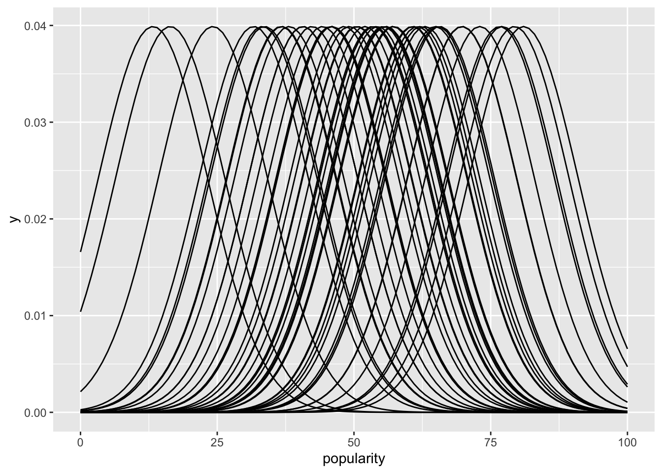
Looks kind of redonkulonk, doesn’t it? That can’t be right. Probably not even useful. But, let’s see how we would have done it anyway.
no_pooled_model <- stan_glm(popularity ~ artist - 1,
  data = spotify,
  prior = normal(50, 2.5, autoscale = T),
  prior_aux = exponential(1, autoscale = T), iter = 10000,
  refresh = FALSE
)

prior_summary(no_pooled_model)
## Priors for model 'no_pooled_model'
## ------
##
## Coefficients
## Specified prior:
## ~ normal(location = [50,50,50,...], scale = [2.5,2.5,2.5,...])
## Adjusted prior:
## ~ normal(location = [50,50,50,...], scale = [325.55,558.97,165.63,...])
##
## Auxiliary (sigma)
## Specified prior:
## ~ exponential(rate = 1)
## Adjusted prior:
## ~ exponential(rate = 0.048)
## ------
## See help('prior_summary.stanreg') for more detailsposterior_vs_prior(no_pooled_model)
Our model with prior specification is
- \(Y|_{\mu_j, \sigma} \sim N(\mu_j, \sigma)\)
- \(\mu_j\) is the mean song popularity for artist \(j\)
- \(\sigma\) is the standard deviation in popularity from song to song, which does not depend on the artist.
- \(\mu_j \sim N(50, s_j)\) we allow a different standard deviation for each prior, but have it fixed at 50. We can see the first few standard deviations for the prior are 325.55 (for Camilo), 558.97 (for Lil Skies), etc.
- \(\sigma \sim \mathrm{Exp}(.048)\)
We use the no intercept model (the artist - 1) for ease of interpretation. Each of the means listed when we use tidy is just the mean of the artist, for example.
broom.mixed::tidy(no_pooled_model, effects = c("fixed", "aux"))## # A tibble: 46 × 3
## term estimate std.error
## <chr> <dbl> <dbl>
## 1 artistCamilo 81.0 4.66
## 2 artistLil Skies 79.4 8.29
## 3 artistCamila Cabello 77.1 2.36
## 4 artistJ. Cole 76.7 3.99
## 5 artistSean Kingston 72.9 9.81
## 6 artistFrank Ocean 69.8 2.21
## 7 artistBeyoncé 69.7 2.82
## 8 artistSufjan Stevens 65.6 8.17
## 9 artistLeón Larregui 65.3 8.13
## 10 artistAlok 64.9 3.18
## # … with 36 more rowsWe visualize the estimations from the model as follows (it would also be informative to plot all of the popularities instead of the mean popularities):
predictions_no <- posterior_predict(
  no_pooled_model,
  newdata = artist_means
)

bayesplot::ppc_intervals(artist_means$popularity,
  yrep = predictions_no,
  prob_outer = 0.80
) +
  ggplot2::scale_x_continuous(
    labels = artist_means$artist,
    breaks = 1:nrow(artist_means)
  ) +
  coord_flip()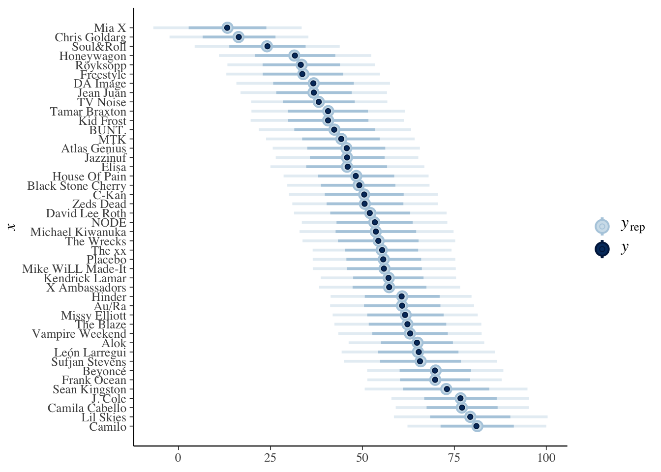
What do the intervals represent in the above plot? Remember, the outer band is the 80 percent posterior predictive interval for songs written by the artist in question. So, for Camilo, we would get:
tidybayes::spread_draws(no_pooled_model, `[\\(a-z].*`, regex = T) %>%
  janitor::clean_names() %>%
  select(artist_camilo, sigma) %>%
  mutate(val = rnorm(n(), artist_camilo, sigma)) %>%
  summarize(HDInterval::hdi(val, credMass = 0.8))
## # A tibble: 2 × 1
## `HDInterval::hdi(val, credMass = 0.8)`
## <dbl>
## 1 61.4
## 2 99.18.3 Partially pooled (hierarchical) model
Recall that \(Y_{ij}\) is the popularity of the \(i\)th song written by artist \(j\). Suppose we observe data consisting of \(n_j\) values of popularity for artist \(j = 1, \ldots, J\). We imagine that the mean popularity of songs for artist \(j\) comes from a normal distribution with mean \(\mu\) and standard deviation \(\sigma_\mu\). We model the popularity of songs on the artist level as normal with mean \(\mu_j\) and common standard deviation \(\sigma_y\). As usual, we would want to find the probability of the parameters given the data \(y_{ij}\), but we can’t do that directly, so we apply Bayes’ rule:
\[ f(\mu, \sigma_\mu, \mu_j, \sigma_y| y_{ij}) \propto f(y_{ij}|\mu, \sigma_\mu, \mu_j, \sigma_y) f(\mu, \sigma_\mu, \mu_j, \sigma_y) \\ = \Pi \mathrm{dnorm}(y_{ij}, \mu_j, \sigma_y) f(\mu_j, \sigma_y|\mu\sigma_\mu) f(\mu, \sigma_\mu)\\ = \Pi \mathrm{dnorm}(y_{ij}, \mu_j, \sigma_y) \Pi \mathrm{dnorm}(\mu_j, \mu, \sigma_\mu) f_1(\mu) f_2(\sigma_\mu) f_3(\sigma_y) \]
where \(f_1\), \(f_2\) and \(f_3\) represent the prior distributions of \(\mu\), \(\sigma_\mu\) and \(\sigma_y\). Note that, as before, we are assuming that once we know \(\mu_j\) and \(\sigma_y\), the distribution of the data does not depend on \(\mu\) and \(\sigma_\mu\).
Let’s see how it looks written a different way.
- \(Y_{ij} \sim N(\mu_j, \sigma_y)\)
- \(\mu_j \sim N(\mu, sigma)\)
- \(\mu\) has a normal prior.
- \(\sigma_\mu\) and \(\sigma_y\) have exponential priors.
We can interpret the parameters of the model as follows:
- \(\mu_j\) is the mean popularity of artist \(j\)
- \(\sigma_y\) is the within artist variability of popularity, common among all artists.
- \(\mu\) is the mean song popularity across all artists; that is, “the mean rating for the most average artist,” as described in the book.
- \(\sigma_\mu\) is the between-group variability. This describes the variation of \(\mu_j\) from artist to artist.
8.3.1 Equivalent Model
We could also have modeled the artist means in terms of their deviations from the overall mean \(\mu\). Let \(b_j\) be the difference between the artist mean \(\mu_j\) and the overall mean \(\mu\), so that \(\mu + b_j = \mu_j\). We would then have the following model:
- \(Y_{ij} \sim N(\mu + b_j, \sigma_y)\)
- \(b_j \sim N(0, \sigma_\mu)\)
- \(\mu\) has a normal prior.
- \(\sigma_\mu\) and \(\sigma_y\) have exponential priors.
8.3.2 Within vs between group variability
The variance in \(Y\), the popularity of songs, breaks down into two components. The within group component, which we denoted as \(\sigma_y^2\) above, and the between groups component, which we denoted as \(\sigma_\mu^2\) above. It is not obviously true, but it is the case that \(\mathrm{Var}(Y) = \sigma_y^2 + \sigma_\mu^2\). That is, the total variance of popularity is the sum of the within group variance and the between group variance.
We can also consider the percentage of the total variance explained by within group variance: \(\frac{\sigma_y^2}{\sigma_y^2 + \sigma_\mu^2}\), as well as the percentage explained by the between group variance. These percentages are numbers between 0 and 1, and we will consider them further in the sequel.
8.4 Posterior Analysis
We start by seeing how to simulate draws from the posterior distribution of the parameters.
spotify_hier <- stan_glmer(popularity ~ (1 | artist),
  data = spotify,
  family = gaussian(),
  prior_intercept = normal(50, 2.5, autoscale = T),
  prior_aux = exponential(1, autoscale = T)
)
##
## SAMPLING FOR MODEL 'continuous' NOW (CHAIN 1).
## Chain 1:
## Chain 1: Gradient evaluation took 0.000123 seconds
## Chain 1: 1000 transitions using 10 leapfrog steps per transition would take 1.23 seconds.
## Chain 1: Adjust your expectations accordingly!
## Chain 1:
## Chain 1:
## Chain 1: Iteration: 1 / 2000 [ 0%] (Warmup)
## Chain 1: Iteration: 200 / 2000 [ 10%] (Warmup)
## Chain 1: Iteration: 400 / 2000 [ 20%] (Warmup)
## Chain 1: Iteration: 600 / 2000 [ 30%] (Warmup)
## Chain 1: Iteration: 800 / 2000 [ 40%] (Warmup)
## Chain 1: Iteration: 1000 / 2000 [ 50%] (Warmup)
## Chain 1: Iteration: 1001 / 2000 [ 50%] (Sampling)
## Chain 1: Iteration: 1200 / 2000 [ 60%] (Sampling)
## Chain 1: Iteration: 1400 / 2000 [ 70%] (Sampling)
## Chain 1: Iteration: 1600 / 2000 [ 80%] (Sampling)
## Chain 1: Iteration: 1800 / 2000 [ 90%] (Sampling)
## Chain 1: Iteration: 2000 / 2000 [100%] (Sampling)
## Chain 1:
## Chain 1: Elapsed Time: 0.731146 seconds (Warm-up)
## Chain 1: 0.604363 seconds (Sampling)
## Chain 1: 1.33551 seconds (Total)
## Chain 1:
##
## SAMPLING FOR MODEL 'continuous' NOW (CHAIN 2).
## Chain 2:
## Chain 2: Gradient evaluation took 2.5e-05 seconds
## Chain 2: 1000 transitions using 10 leapfrog steps per transition would take 0.25 seconds.
## Chain 2: Adjust your expectations accordingly!
## Chain 2:
## Chain 2:
## Chain 2: Iteration: 1 / 2000 [ 0%] (Warmup)
## Chain 2: Iteration: 200 / 2000 [ 10%] (Warmup)
## Chain 2: Iteration: 400 / 2000 [ 20%] (Warmup)
## Chain 2: Iteration: 600 / 2000 [ 30%] (Warmup)
## Chain 2: Iteration: 800 / 2000 [ 40%] (Warmup)
## Chain 2: Iteration: 1000 / 2000 [ 50%] (Warmup)
## Chain 2: Iteration: 1001 / 2000 [ 50%] (Sampling)
## Chain 2: Iteration: 1200 / 2000 [ 60%] (Sampling)
## Chain 2: Iteration: 1400 / 2000 [ 70%] (Sampling)
## Chain 2: Iteration: 1600 / 2000 [ 80%] (Sampling)
## Chain 2: Iteration: 1800 / 2000 [ 90%] (Sampling)
## Chain 2: Iteration: 2000 / 2000 [100%] (Sampling)
## Chain 2:
## Chain 2: Elapsed Time: 0.728449 seconds (Warm-up)
## Chain 2: 0.414264 seconds (Sampling)
## Chain 2: 1.14271 seconds (Total)
## Chain 2:
##
## SAMPLING FOR MODEL 'continuous' NOW (CHAIN 3).
## Chain 3:
## Chain 3: Gradient evaluation took 2.1e-05 seconds
## Chain 3: 1000 transitions using 10 leapfrog steps per transition would take 0.21 seconds.
## Chain 3: Adjust your expectations accordingly!
## Chain 3:
## Chain 3:
## Chain 3: Iteration: 1 / 2000 [ 0%] (Warmup)
## Chain 3: Iteration: 200 / 2000 [ 10%] (Warmup)
## Chain 3: Iteration: 400 / 2000 [ 20%] (Warmup)
## Chain 3: Iteration: 600 / 2000 [ 30%] (Warmup)
## Chain 3: Iteration: 800 / 2000 [ 40%] (Warmup)
## Chain 3: Iteration: 1000 / 2000 [ 50%] (Warmup)
## Chain 3: Iteration: 1001 / 2000 [ 50%] (Sampling)
## Chain 3: Iteration: 1200 / 2000 [ 60%] (Sampling)
## Chain 3: Iteration: 1400 / 2000 [ 70%] (Sampling)
## Chain 3: Iteration: 1600 / 2000 [ 80%] (Sampling)
## Chain 3: Iteration: 1800 / 2000 [ 90%] (Sampling)
## Chain 3: Iteration: 2000 / 2000 [100%] (Sampling)
## Chain 3:
## Chain 3: Elapsed Time: 0.729909 seconds (Warm-up)
## Chain 3: 0.579332 seconds (Sampling)
## Chain 3: 1.30924 seconds (Total)
## Chain 3:
##
## SAMPLING FOR MODEL 'continuous' NOW (CHAIN 4).
## Chain 4:
## Chain 4: Gradient evaluation took 2.2e-05 seconds
## Chain 4: 1000 transitions using 10 leapfrog steps per transition would take 0.22 seconds.
## Chain 4: Adjust your expectations accordingly!
## Chain 4:
## Chain 4:
## Chain 4: Iteration: 1 / 2000 [ 0%] (Warmup)
## Chain 4: Iteration: 200 / 2000 [ 10%] (Warmup)
## Chain 4: Iteration: 400 / 2000 [ 20%] (Warmup)
## Chain 4: Iteration: 600 / 2000 [ 30%] (Warmup)
## Chain 4: Iteration: 800 / 2000 [ 40%] (Warmup)
## Chain 4: Iteration: 1000 / 2000 [ 50%] (Warmup)
## Chain 4: Iteration: 1001 / 2000 [ 50%] (Sampling)
## Chain 4: Iteration: 1200 / 2000 [ 60%] (Sampling)
## Chain 4: Iteration: 1400 / 2000 [ 70%] (Sampling)
## Chain 4: Iteration: 1600 / 2000 [ 80%] (Sampling)
## Chain 4: Iteration: 1800 / 2000 [ 90%] (Sampling)
## Chain 4: Iteration: 2000 / 2000 [100%] (Sampling)
## Chain 4:
## Chain 4: Elapsed Time: 0.661534 seconds (Warm-up)
## Chain 4: 0.528148 seconds (Sampling)
## Chain 4: 1.18968 seconds (Total)
## Chain 4:We can see that we set the prior for \(\mu\) to be normal with mean 50, and the prior for \(\sigma_\mu\) to be exponential. We are using the second version of the model, so we don’t need to specify the means of the priors for the \(\mu_j\); the means of the priors of the \(b_j\) will just be 0. We did not set the prior for the within-group variation, choosing to let rstanarm do that automatically for us.
prior_summary(spotify_hier)## Priors for model 'spotify_hier'
## ------
## Intercept (after predictors centered)
## Specified prior:
## ~ normal(location = 50, scale = 2.5)
## Adjusted prior:
## ~ normal(location = 50, scale = 52)
##
## Auxiliary (sigma)
## Specified prior:
## ~ exponential(rate = 1)
## Adjusted prior:
## ~ exponential(rate = 0.048)
##
## Covariance
## ~ decov(reg. = 1, conc. = 1, shape = 1, scale = 1)
## ------
## See help('prior_summary.stanreg') for more detailsAnd this is why; the specification for the within-group variation is a bit strange, and will be discussed later when it makes more sense. Currently, we just assume that this is a reasonable weakly informative prior.
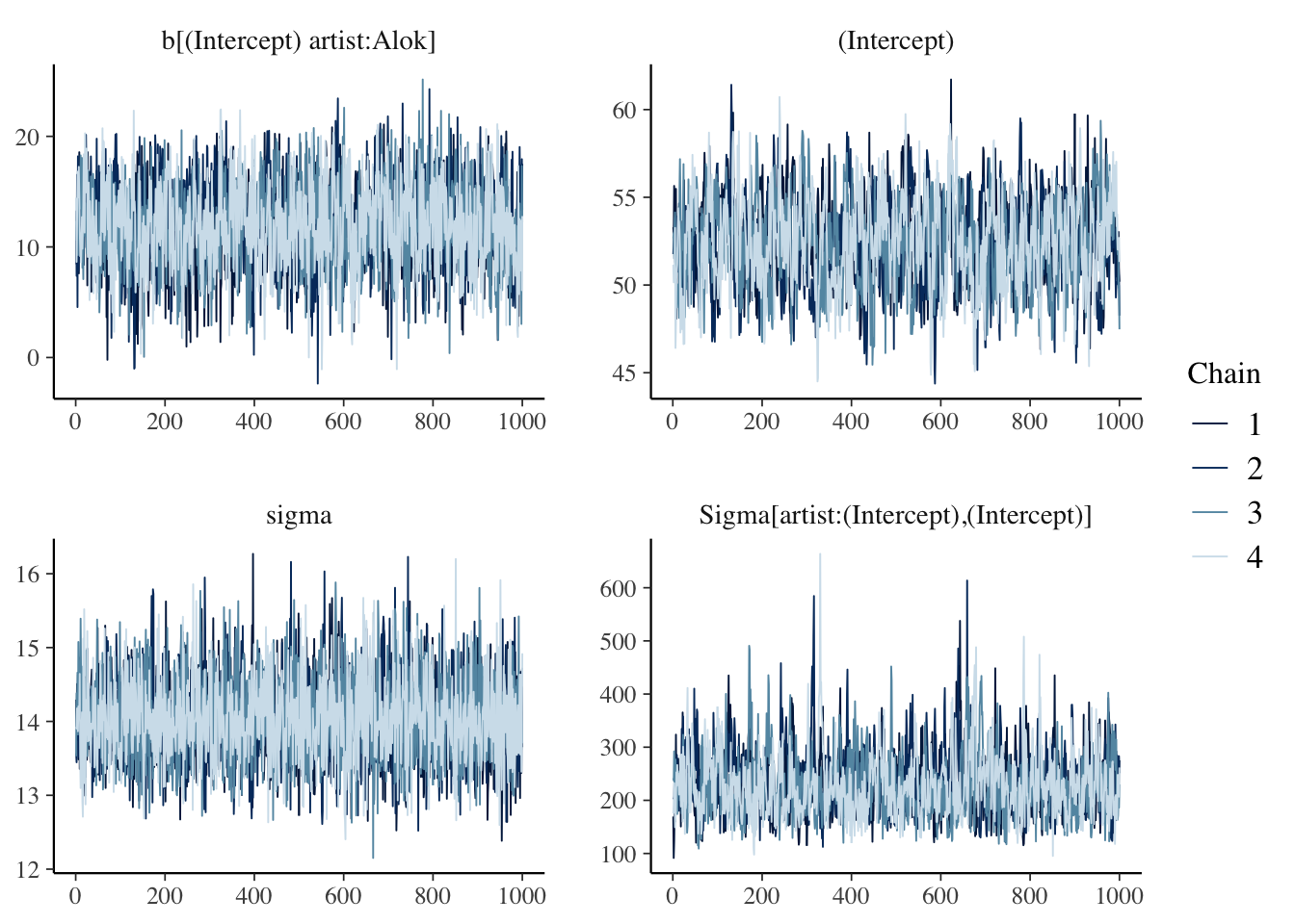
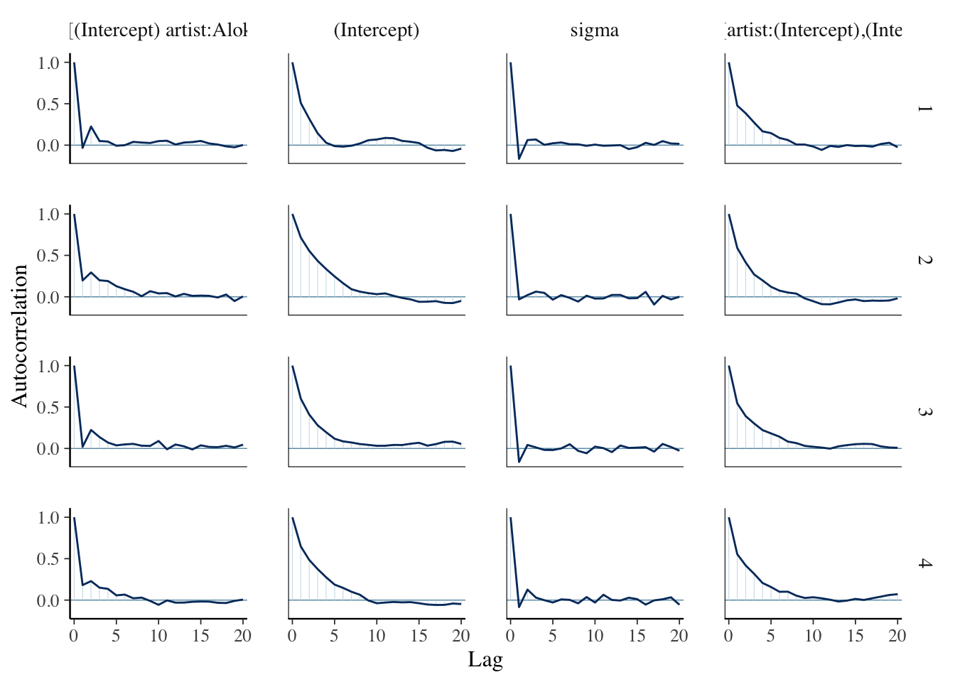
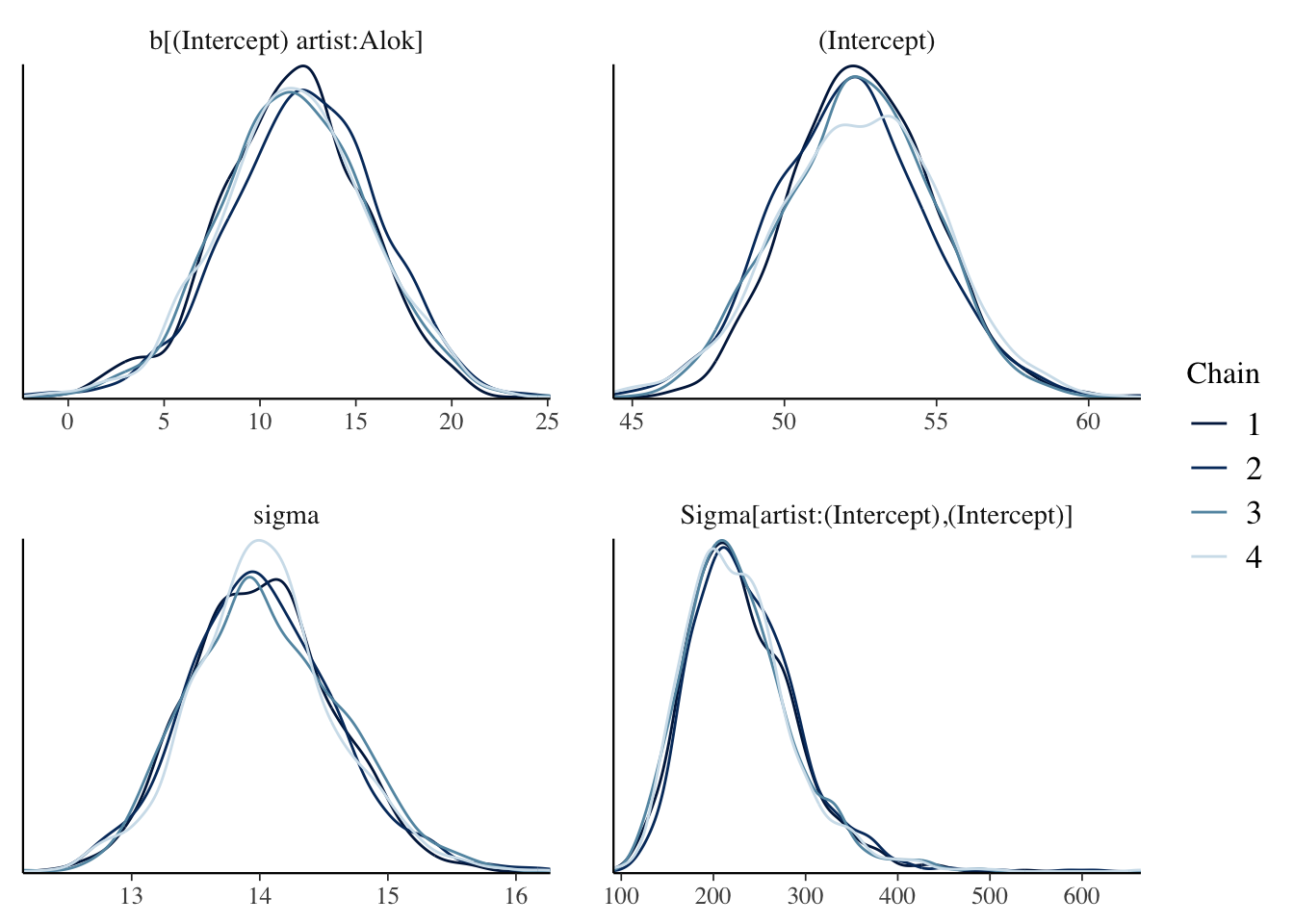
Let’s check some convergence diagnostics for one of the \(b_j\) and
library(bayesplot)
tidybayes::get_variables(spotify_hier)
## [1] "(Intercept)"
## [2] "b[(Intercept) artist:Camilo]"
## [3] "b[(Intercept) artist:Lil_Skies]"
## [4] "b[(Intercept) artist:Camila_Cabello]"
## [5] "b[(Intercept) artist:J._Cole]"
## [6] "b[(Intercept) artist:Sean_Kingston]"
## [7] "b[(Intercept) artist:Frank_Ocean]"
## [8] "b[(Intercept) artist:Beyoncé]"
## [9] "b[(Intercept) artist:Sufjan_Stevens]"
## [10] "b[(Intercept) artist:León_Larregui]"
## [11] "b[(Intercept) artist:Alok]"
## [12] "b[(Intercept) artist:Vampire_Weekend]"
## [13] "b[(Intercept) artist:The_Blaze]"
## [14] "b[(Intercept) artist:Missy_Elliott]"
## [15] "b[(Intercept) artist:Au/Ra]"
## [16] "b[(Intercept) artist:Hinder]"
## [17] "b[(Intercept) artist:X_Ambassadors]"
## [18] "b[(Intercept) artist:Kendrick_Lamar]"
## [19] "b[(Intercept) artist:Mike_WiLL_Made-It]"
## [20] "b[(Intercept) artist:Placebo]"
## [21] "b[(Intercept) artist:The_xx]"
## [22] "b[(Intercept) artist:The_Wrecks]"
## [23] "b[(Intercept) artist:Michael_Kiwanuka]"
## [24] "b[(Intercept) artist:NODE]"
## [25] "b[(Intercept) artist:David_Lee_Roth]"
## [26] "b[(Intercept) artist:Zeds_Dead]"
## [27] "b[(Intercept) artist:C-Kan]"
## [28] "b[(Intercept) artist:Black_Stone_Cherry]"
## [29] "b[(Intercept) artist:House_Of_Pain]"
## [30] "b[(Intercept) artist:Elisa]"
## [31] "b[(Intercept) artist:Jazzinuf]"
## [32] "b[(Intercept) artist:Atlas_Genius]"
## [33] "b[(Intercept) artist:MTK]"
## [34] "b[(Intercept) artist:BUNT.]"
## [35] "b[(Intercept) artist:Kid_Frost]"
## [36] "b[(Intercept) artist:Tamar_Braxton]"
## [37] "b[(Intercept) artist:TV_Noise]"
## [38] "b[(Intercept) artist:Jean_Juan]"
## [39] "b[(Intercept) artist:DA_Image]"
## [40] "b[(Intercept) artist:Freestyle]"
## [41] "b[(Intercept) artist:Röyksopp]"
## [42] "b[(Intercept) artist:Honeywagon]"
## [43] "b[(Intercept) artist:Soul&Roll]"
## [44] "b[(Intercept) artist:Chris_Goldarg]"
## [45] "b[(Intercept) artist:Mia_X]"
## [46] "sigma"
## [47] "Sigma[artist:(Intercept),(Intercept)]"
## [48] "accept_stat__"
## [49] "stepsize__"
## [50] "treedepth__"
## [51] "n_leapfrog__"
## [52] "divergent__"
## [53] "energy__"mcmc_trace(spotify_hier, pars = c(
"b[(Intercept) artist:Alok]",
"(Intercept)",
"sigma",
"Sigma[artist:(Intercept),(Intercept)]"
))
mcmc_acf(spotify_hier, pars = c(
  "b[(Intercept) artist:Alok]",
  "(Intercept)",
  "sigma",
  "Sigma[artist:(Intercept),(Intercept)]"
))
mcmc_dens_overlay(spotify_hier, pars = c(
  "b[(Intercept) artist:Alok]",
  "(Intercept)",
  "sigma",
  "Sigma[artist:(Intercept),(Intercept)]"
))
neff_ratio(spotify_hier, pars = c(
  "b[(Intercept) artist:Alok]",
  "(Intercept)",
  "sigma",
  "Sigma[artist:(Intercept),(Intercept)]"
))
## (Intercept)
## 0.18850
## b[(Intercept) artist:Alok]
## 0.34075
## sigma
## 1.01350
## Sigma[artist:(Intercept),(Intercept)]
## 0.21350rhat(spotify_hier, pars = c(
"b[(Intercept) artist:Alok]",
"(Intercept)",
"sigma",
"Sigma[artist:(Intercept),(Intercept)]"
))## (Intercept)
## 1.0018017
## b[(Intercept) artist:Alok]
## 1.0015923
## sigma
## 0.9995779
## Sigma[artist:(Intercept),(Intercept)]
## 1.0028074Let’s check the posterior predictive density versus the observed density of the popularitoes. It’s not terrible; could be better, but it definitely follows more or less the right shape.
pp_check(spotify_hier)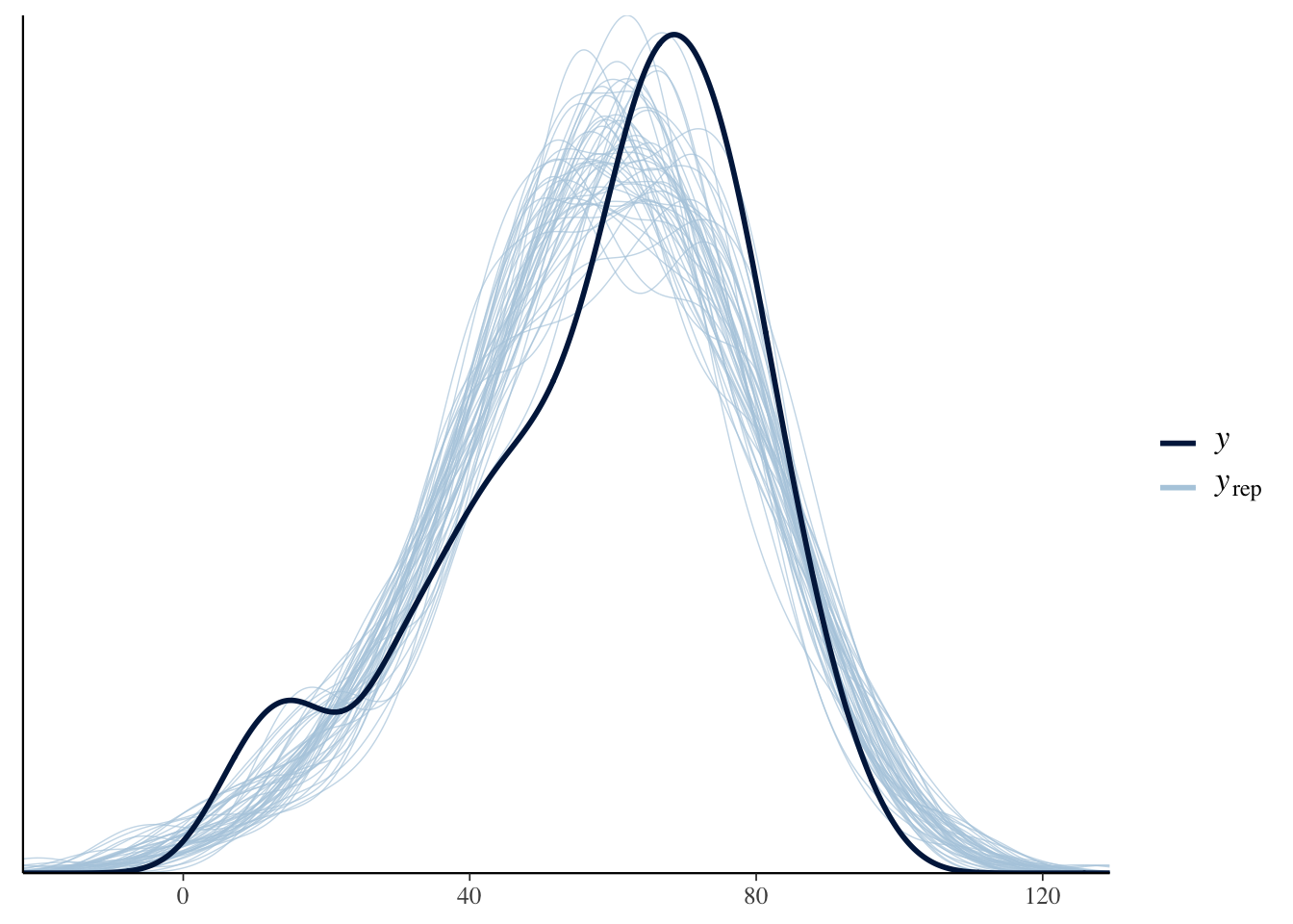
Now, let’s return to the parameters that we saw from get_Variables. That was quite the list!!! Let’s go through them to understand what they are refering to.
- \(\mu\) =
(Intercept) - standard deviation within group = \(\sigma_y\) =
sigma - variance between groups = \(\sigma_\mu^2\) =
Sigma[artist:(Intercept),(Intercept)]
We can get the estimates, standard errors and confindence intervals for these using tidy:
broom.mixed::tidy(spotify_hier,
  effects = c("fixed", "ran_par"),
  conf.int = TRUE,
  conf.level = .8
)
## # A tibble: 3 × 6
## term estimate std.error conf.low conf.high group
## <chr> <dbl> <dbl> <dbl> <dbl> <chr>
## 1 (Intercept) 52.4 2.51 49.3 55.5 <NA>
## 2 sd_(Intercept).artist 15.2 NA NA NA artist
## 3 sd_Observation.Residual 14.0 NA NA NA ResidualWe see that our estimate for the mean of artist means is 52.5, and we think it is somewhere between 49.4 and 55.8. Note that this is similar to what t.test gives when we find the 80 percent confidence interval for the mean of the artist means. It is not similar to what t.test gives when we supply the popularity of all songs.
spotify %>%
  group_by(artist) %>%
  summarize(mu = mean(popularity)) %>%
  with(t.test(mu, conf.level = .8))
##
## One Sample t-test
##
## data: mu
## t = 21.764, df = 43, p-value < 2.2e-16
## alternative hypothesis: true mean is not equal to 0
## 80 percent confidence interval:
## 49.00667 55.24105
## sample estimates:
## mean of x
## 52.12386t.test(spotify$popularity, conf.level = .8) # this isn't it##
## One Sample t-test
##
## data: spotify$popularity
## t = 52.935, df = 349, p-value < 2.2e-16
## alternative hypothesis: true mean is not equal to 0
## 80 percent confidence interval:
## 56.98624 59.81948
## sample estimates:
## mean of x
## 58.40286Finally, looking at the standard deviation estimates, we see that \(\sigma_y \approx 14\), which means we expect the popularity of songs within the same artist to vary by about plus or minus 28. The standard deviation between groups is a little bit higher, 15.1. This means that \(\frac{15.1^2}{15.1^2 + 14^2} = 54\%\) of the variance in popularity is explained by the between groups variance, while 46 percent of the variance in popularity is explained by the within-artist variance.
8.4.1 Two examples of posterior prediction
Find an 80 percent posterior prediction interval for a song by Beyonce.
The uncertainty in the popularity of a new song by Beyonce comes from two sources. First, the uncertainty in our estimates for \(\mu_j\) and \(\sigma_y\), and second, from the range of popularities in the songs themselves.
Here’s how we can do it.
library(tidybayes)
spread_draws(spotify_hier, `[\\(a-zA-Z].*`, regex = T) %>%
  janitor::clean_names() %>%
  select(matches("Sigm|sig|^int|beyonc")) %>%
  mutate(pop = rnorm(n(), intercept + b_intercept_artist_beyonce, sigma)) %>%
  summarize(HDInterval::hdi(pop, credMass = 0.8))
## # A tibble: 2 × 1
## `HDInterval::hdi(pop, credMass = 0.8)`
## <dbl>
## 1 51.9
## 2 88.8Find an 80 percent posterior prediction interval for a song by Early B.
This time, there is uncertainty from three sources:
- The uncertainty in our estimates of the parameters.
- The variation of popularity within an artist.
- The variation of popularity of songs between artists.
spread_draws(spotify_hier, `[\\(a-zA-Z].*`, regex = T) %>%
  janitor::clean_names() %>%
  select(matches("Sigm|sig|^int")) %>%
  mutate(sigma_artist = sqrt(sigma_artist_intercept_intercept)) %>%
  mutate(
    artist_mean = rnorm(n(), intercept, sigma_artist),
    pop = rnorm(n(), artist_mean, sigma)
  ) %>%
  summarize(HDInterval::hdi(pop, credMass = 0.8))
## # A tibble: 2 × 1
## `HDInterval::hdi(pop, credMass = 0.8)`
## <dbl>
## 1 24.4
## 2 77.78.5 Shrinkage
Shrinkage describes the phenomenon in a hierarchical model, the parameter estimates tend to be closer to each other than they would be in a non-pooled model. To see that, let’s compare the distribution of artist means in the hierarchical model to those from the non-pooled model we did earlier.
get_variables(no_pooled_model)## [1] "artistCamilo" "artistLil Skies"
## [3] "artistCamila Cabello" "artistJ. Cole"
## [5] "artistSean Kingston" "artistFrank Ocean"
## [7] "artistBeyoncé" "artistSufjan Stevens"
## [9] "artistLeón Larregui" "artistAlok"
## [11] "artistVampire Weekend" "artistThe Blaze"
## [13] "artistMissy Elliott" "artistAu/Ra"
## [15] "artistHinder" "artistX Ambassadors"
## [17] "artistKendrick Lamar" "artistMike WiLL Made-It"
## [19] "artistPlacebo" "artistThe xx"
## [21] "artistThe Wrecks" "artistMichael Kiwanuka"
## [23] "artistNODE" "artistDavid Lee Roth"
## [25] "artistZeds Dead" "artistC-Kan"
## [27] "artistBlack Stone Cherry" "artistHouse Of Pain"
## [29] "artistElisa" "artistJazzinuf"
## [31] "artistAtlas Genius" "artistMTK"
## [33] "artistBUNT." "artistKid Frost"
## [35] "artistTamar Braxton" "artistTV Noise"
## [37] "artistJean Juan" "artistDA Image"
## [39] "artistFreestyle" "artistRöyksopp"
## [41] "artistHoneywagon" "artistSoul&Roll"
## [43] "artistChris Goldarg" "artistMia X"
## [45] "sigma" "accept_stat__"
## [47] "stepsize__" "treedepth__"
## [49] "n_leapfrog__" "divergent__"
## [51] "energy__"spread_draws(no_pooled_model, `^artist.*`, regex = T) %>%
summarize(across(matches("^artist"), mean)) %>%
t() %>%
sd()## [1] 15.88599get_variables(spotify_hier)## [1] "(Intercept)"
## [2] "b[(Intercept) artist:Camilo]"
## [3] "b[(Intercept) artist:Lil_Skies]"
## [4] "b[(Intercept) artist:Camila_Cabello]"
## [5] "b[(Intercept) artist:J._Cole]"
## [6] "b[(Intercept) artist:Sean_Kingston]"
## [7] "b[(Intercept) artist:Frank_Ocean]"
## [8] "b[(Intercept) artist:Beyoncé]"
## [9] "b[(Intercept) artist:Sufjan_Stevens]"
## [10] "b[(Intercept) artist:León_Larregui]"
## [11] "b[(Intercept) artist:Alok]"
## [12] "b[(Intercept) artist:Vampire_Weekend]"
## [13] "b[(Intercept) artist:The_Blaze]"
## [14] "b[(Intercept) artist:Missy_Elliott]"
## [15] "b[(Intercept) artist:Au/Ra]"
## [16] "b[(Intercept) artist:Hinder]"
## [17] "b[(Intercept) artist:X_Ambassadors]"
## [18] "b[(Intercept) artist:Kendrick_Lamar]"
## [19] "b[(Intercept) artist:Mike_WiLL_Made-It]"
## [20] "b[(Intercept) artist:Placebo]"
## [21] "b[(Intercept) artist:The_xx]"
## [22] "b[(Intercept) artist:The_Wrecks]"
## [23] "b[(Intercept) artist:Michael_Kiwanuka]"
## [24] "b[(Intercept) artist:NODE]"
## [25] "b[(Intercept) artist:David_Lee_Roth]"
## [26] "b[(Intercept) artist:Zeds_Dead]"
## [27] "b[(Intercept) artist:C-Kan]"
## [28] "b[(Intercept) artist:Black_Stone_Cherry]"
## [29] "b[(Intercept) artist:House_Of_Pain]"
## [30] "b[(Intercept) artist:Elisa]"
## [31] "b[(Intercept) artist:Jazzinuf]"
## [32] "b[(Intercept) artist:Atlas_Genius]"
## [33] "b[(Intercept) artist:MTK]"
## [34] "b[(Intercept) artist:BUNT.]"
## [35] "b[(Intercept) artist:Kid_Frost]"
## [36] "b[(Intercept) artist:Tamar_Braxton]"
## [37] "b[(Intercept) artist:TV_Noise]"
## [38] "b[(Intercept) artist:Jean_Juan]"
## [39] "b[(Intercept) artist:DA_Image]"
## [40] "b[(Intercept) artist:Freestyle]"
## [41] "b[(Intercept) artist:Röyksopp]"
## [42] "b[(Intercept) artist:Honeywagon]"
## [43] "b[(Intercept) artist:Soul&Roll]"
## [44] "b[(Intercept) artist:Chris_Goldarg]"
## [45] "b[(Intercept) artist:Mia_X]"
## [46] "sigma"
## [47] "Sigma[artist:(Intercept),(Intercept)]"
## [48] "accept_stat__"
## [49] "stepsize__"
## [50] "treedepth__"
## [51] "n_leapfrog__"
## [52] "divergent__"
## [53] "energy__"spread_draws(spotify_hier, `^b.*|^\\(.*`, regex = T) %>%
janitor::clean_names() %>%
summarize(across(matches("^b"), function(x) mean(x + intercept))) %>%
t() %>%
sd()## [1] 13.62124We see that the estimated means for the hierachical model have lower standard deviation than the means for the no pooled model. This is because the artist means have been pulled toward the overall mean of artists. Here is another plot we can use to look at it, from the book. We see that the posterior predictive intervals are pulled closer to the group means, so that the artists with low means are pulled up, while those with high means are pulled down.
predictions_hierarchical <- posterior_predict(spotify_hier,
  newdata = artist_means
)

ppc_intervals(artist_means$popularity, yrep = predictions_hierarchical) +
  scale_x_continuous(
    labels = artist_means$artist,
    breaks = 1:nrow(artist_means)
  ) +
  coord_flip()