Chapter 5 Count Models
In this chapter, we discuss models for count data such that, for example, \(Y|X = x\) is reasonably modeled by a Poisson random variable.
Let’s remind ourselves about the Gaussian regression model. We are modeling the expected outcome at \(X = x\) by \(\beta_0 + \beta_1 x\), and we are assuming that the error in that model is normal with mean \(\sigma\) that doesn’t depend on \(x\).
Let’s do a similar thing with Poisson. Let’s assume that we have data in the form \((x_1, y_1), \ldots, (x_n, y_n)\), where the \(x_i\) are either non-random or we are not modeling the randomness in them. The \(y_i\) are observations of a Poisson random variable \(Y_i\) with mean \(\lambda_i\). We write \(Y|\lambda_i \sim \mathrm{Pois}(\lambda_i)\). Now, might think that we should model the expected outcome at \(X = x\) by \(\beta_0 + \beta_1 x\), and since Poisson is a single parameter random variable, the variance at \(X = x\) would be assumed to be \(\beta_0 + \beta_1 x\). There is nothing inherently wrong with this. However, it can lead to some odd cases where \(\beta_0 + \beta_1 x < 0\), which doesn’t make sense for the expected value of a Poisson random variable.
Instead, we choose to model the log of the mean of the response at \(X = x\) by \(\beta_0 + \beta_1 x\). That is, \(\log E[Y_i|X = x] = \beta_0 + \beta_1 x\). Alternatively, we are modeling \(\log \lambda_i = \beta_0 + \beta_1 x\) or \(\lambda_i = \exp (\beta_0 + \beta_1 x)\).
Let’s look at an example, after which we will talk about setting priors and completely specifying the model.
Let’s return to the number of soccer players born on each day of the year. We say previously that though it looked linear, giving it a linear fit with Gaussian error led to posterior prediction intervals that were sometimes negative. That’s not the best.
remotes::install_github(repo = "speegled/bayeta")soccer <- bayeta::soccerNow, we model it according to \(\log \lambda_i = \beta_0 + \beta_1 x_i\), and \(Y \sim \mathrm{Pois}(\lambda_i)\).
soccer_model <- rstanarm::stan_glm(count ~ day_no_dual,
  data = soccer,
  family = poisson(link = "log"),
  refresh = 0
)


rstanarm::prior_summary(soccer_model)
## Priors for model 'soccer_model'
## ------
## Intercept (after predictors centered)
## ~ normal(location = 0, scale = 2.5)
##
## Coefficients
## Specified prior:
## ~ normal(location = 0, scale = 2.5)
## Adjusted prior:
## ~ normal(location = 0, scale = 0.024)
## ------
## See help('prior_summary.stanreg') for more detailsbroom.mixed::tidy(soccer_model)## # A tibble: 2 × 3
## term estimate std.error
## <chr> <dbl> <dbl>
## 1 (Intercept) 3.27 0.0231
## 2 day_no_dual -0.00220 0.000123We see that the model for the mean number of people born on day \(x\) is given by \(e^{3.27 + -0.00220 x}\), where \(x\) is the (cohort) day of year. If we visualize this, it looks pretty good:
library(tidyverse)
ggplot(soccer, aes(x = day_no_dual, y = count)) +
  geom_point() +
  geom_function(fun = function(x) exp(3.27 + -0.00220 * x))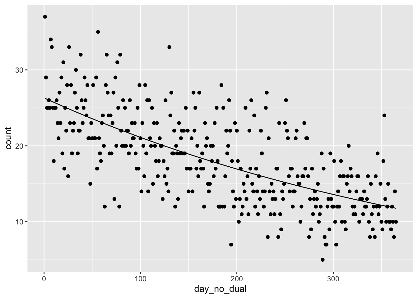
Suppose we want a 99 percent posterior prediction interval for number of players born on day 365. Recall that this included negative numbers i n our previous model. We would use spread_draws and rpois rather than rnorm, because we are modeling the error as Poisson.
tidybayes::spread_draws(soccer_model, `[\\(a-z].*`, regex = T) %>%
  janitor::clean_names() %>%
  mutate(val = rpois(n(), exp(intercept + day_no_dual * 365))) %>%
  summarize(hdi = HDInterval::hdi(val, credMass = 0.99))
## # A tibble: 2 × 1
## hdi
## <int>
## 1 4
## 2 20We see that the 99 percent posterior prediction interval is \([5, 21]\), which is quite different than the \([-1, 21]\) interval we got with a Gaussian model.
We end by computing a 95 percent credible interval for the mean number of players born on the 200th day.
library(tidybayes)
spread_draws(soccer_model, `[\\(a-z].*`, regex = T) %>%
  janitor::clean_names() %>%
  mutate(val = exp(intercept + day_no_dual * 200)) %>%
  summarize(hdi = HDInterval::hdi(val, credMass = 0.95))
## # A tibble: 2 × 1
## hdi
## <dbl>
## 1 16.6
## 2 17.5Now that we have seen how it works, let’s take a deeper dive into the model. We have \(Y_i|\beta_0, \beta_1 \sim \mathrm{Pois}(\lambda_i)\) and \(\log \lambda_i = \beta_0 + \beta_1 x_i\). It remains to find reasonable priors for \(\beta_0\) and \(\beta_1\). Note that the priors on the coefficients don’t need to be Poisson for any reason; we chose normal priors in the simple linear regression chapter for convenience. Before we can do that, we probably need to be able to interpret the coefficients.
We have \(\lambda = e^{\beta_0 + \beta_1 x}\), so when \(x = 0\), \(\lambda = e^{\beta_0}\). A good estimate for \(\beta_0\) would then be the log of the average of the \(Y\) values when \(x = 0\). Looking at the plot of data, we could plausibly think the log of the mean at \(x = 0\) could be anywhere between \(\log 15\) and \(\log 35\). So, perhaps a normal prior on \(\beta_0\) with mean 3.1 and standard deviation about 0.3 would be reasonable. The interpretation of \(\beta_1\) is trickier. If we increase \(x\) by one unit, then \(\lambda\) increases by a multiplicative factor of \(e^{\beta_1}\); that is, \(e^{\beta_0 + \beta_1(x + 1)} = e^{\beta_1}e^{\beta_0 + \beta_1 x}\). To estimate \(\beta_1\) in our case, it is probably easier to look at a change of 100. Looking at the plot of points (without the line of fit), it seems like the mean might decrease from about 25 to about 20 when day of birth goes from 0 to 100. That means \(20/25 \approx e^{100\beta_1}\), which solving for \(\beta_1\) gives us \(\beta_1 \approx -0.002\). A worst case decrease might be decreasing from mean 30 at age 0 to mean 15 at age 100, which would lead to an approximation of \(\beta_1 \approx -.007\). So, we could try a normal prior on \(\beta_1\) with mean 0 and standard deviation .005.
rstanarm centers the predictors, which leads to different results, and it also chose much less informative priors based on the summary:
rstanarm::prior_summary(soccer_model)## Priors for model 'soccer_model'
## ------
## Intercept (after predictors centered)
## ~ normal(location = 0, scale = 2.5)
##
## Coefficients
## Specified prior:
## ~ normal(location = 0, scale = 2.5)
## Adjusted prior:
## ~ normal(location = 0, scale = 0.024)
## ------
## See help('prior_summary.stanreg') for more detailsLet’s plot a bunch of posterior lines on the same plot as our data. This is a bit tricky to do, as many things you would naturally try do not work.
lines <- spread_draws(soccer_model, `[\\(a-z].*`, regex = T, ndraws = 100) %>%
  janitor::clean_names()

lines_plot <- lapply(1:100, function(i) {
  geom_function(fun = function(x) exp(lines$intercept[i] + lines$day_no_dual[i] * x), color = "red", alpha = .2)
})

ggplot(soccer, aes(x = day_no_dual, y = count)) +
  geom_point() +
  lines_plot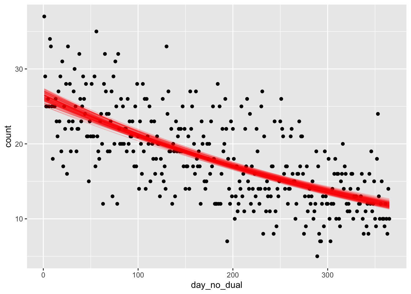
And if we want to see how our posterior estimates compare to the prior:
rstanarm::posterior_vs_prior(soccer_model, pars = "(Intercept)")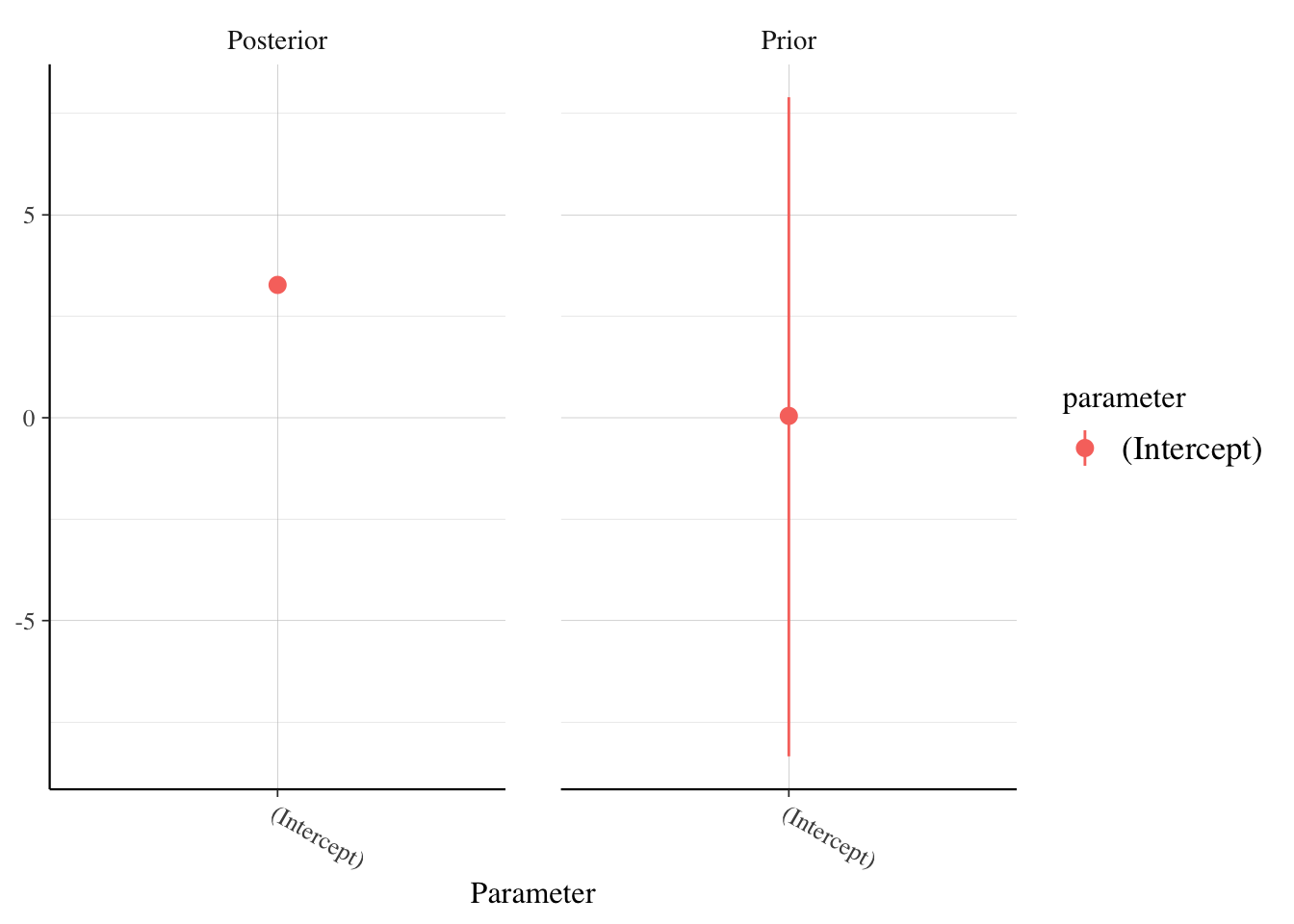
rstanarm::posterior_vs_prior(soccer_model, pars = "day_no_dual")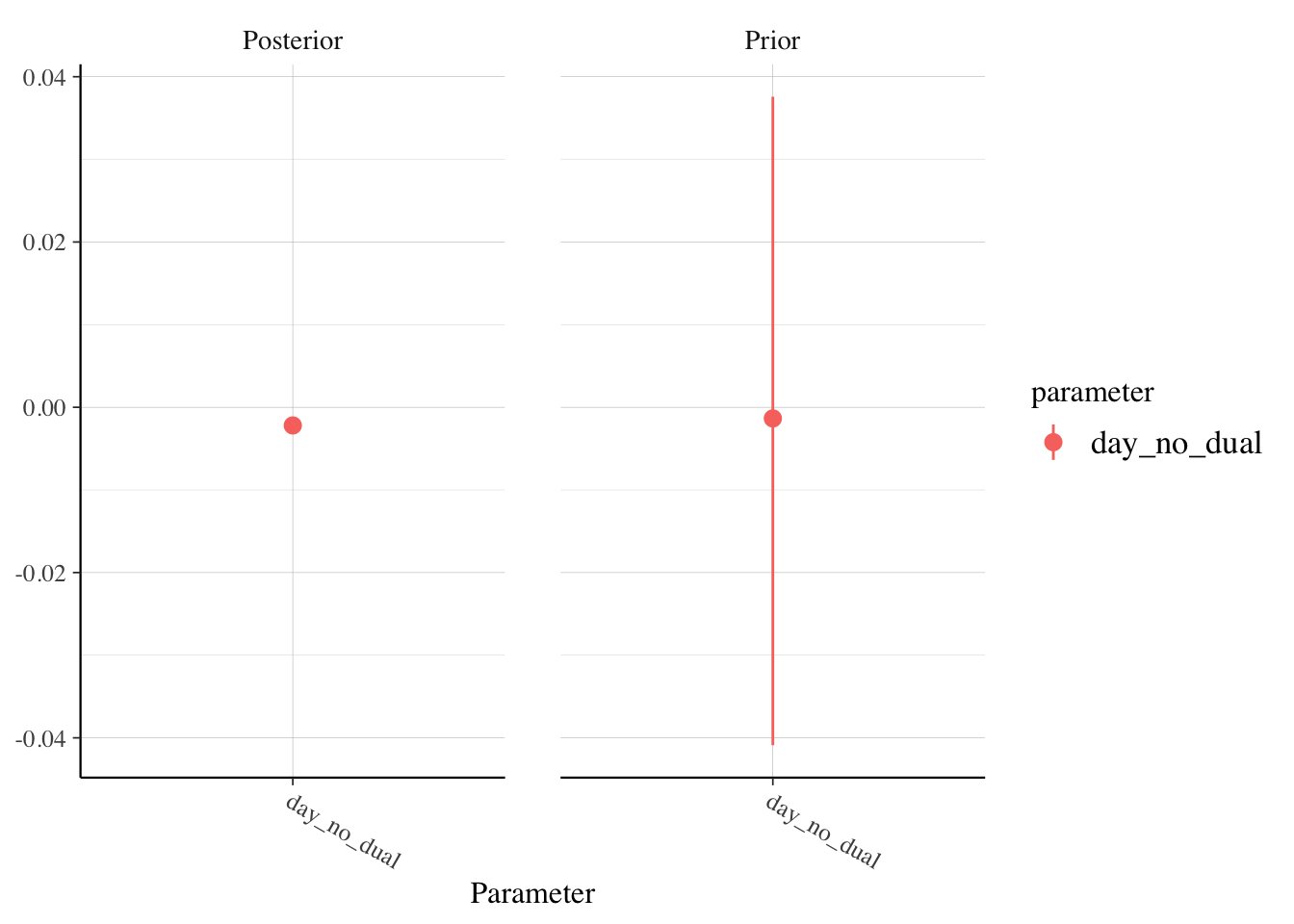
Now, let’s check the posterior predictive distribution versus the actual distribution:
bayesplot::pp_check(soccer_model)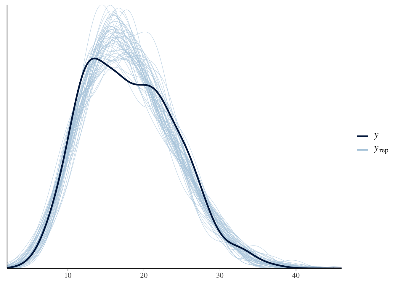
That looks pretty good. Notice how the posterior predictive curves seem to contain the true curve over most values. There is perhaps something weird going on around 18-22, but it doesn’t seem like a red flag to me.
We also had an assumption that the variance of the count should be roughly equal to the mean of the count. How do we check that? One way would be to use a more flexible model which allows for that not to be true, and let the data inform us of whether the variance is equal to the mean. See Negative Binomial Regression below.
Here, we try to assess it directly by plotting the residuals versus fitted.
plot(fitted(soccer_model), resid(soccer_model))
curve(sqrt(x), add = T)
curve(2 * sqrt(x), add = T, lty = 2, col = 2)
curve(-sqrt(x), add = T)
curve(-2 * sqrt(x), add = T, lty = 2, col = 2)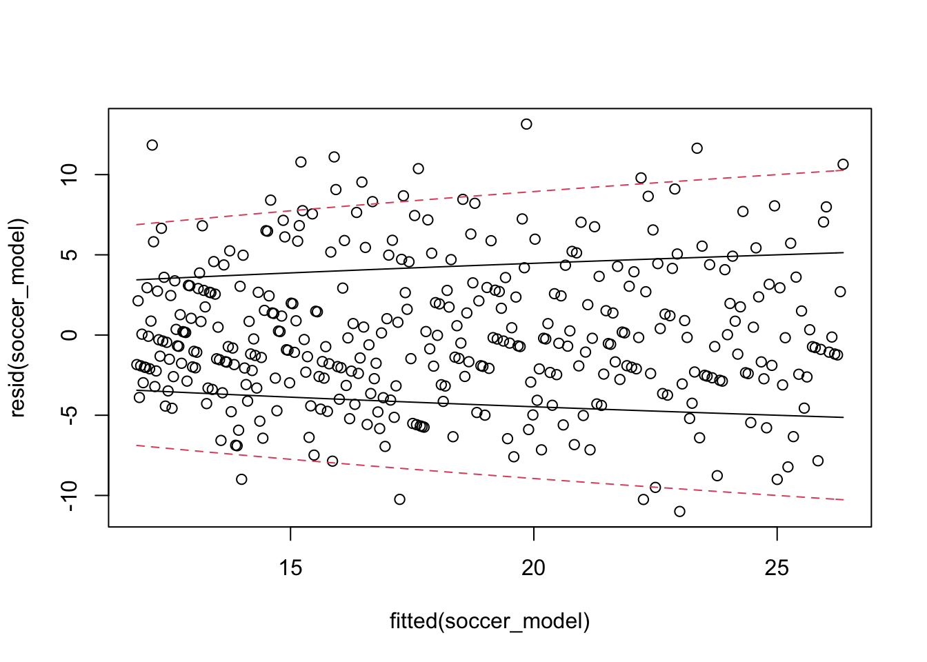
It is hard to see whether the standard deviation of the errors is approximately the square root of the fitted values, but there also doesn’t seem to be compelling evidence that this is not the case. Finally, let’s group the data into 5 groups and compute the mean and variance within the groups to see whether the mean seems approximately equal to the variance.
soccer %>%
  group_by(cut(day_no_dual, 5)) %>%
  summarize(
    mu = mean(count),
    var = var(count)
  )
## # A tibble: 5 × 3
## `cut(day_no_dual, 5)` mu var
## <fct> <dbl> <dbl>
## 1 (0.636,73.8] 24.2 25.5
## 2 (73.8,147] 20.9 20.8
## 3 (147,219] 17.8 23.9
## 4 (219,292] 15.1 22.4
## 5 (292,365] 12.8 11.05.1 Negative Binomial Regression
In this chapter, we see a more flexible model which allows for the variance to be larger than the mean. We will use the negative binomial distribution. This distribution is typically introduced as modeling the number of failures before the \(k\)th success occurs in Bernoulli trials with probability success \(p\). The distribution has two parameters, \(k\) and \(p\). The geometric distribution, which models the number of failures before the 1st success is a speical case, with \(k = 1\).
In our case, we normally don’t have reason to conceptualize the response as a count of successes before the \(k\)th failure, so the parameters become hard to interpret. We re-parameterize the model in terms of \(\mu\), the mean, and size, the dispersion parameter. The probability of success is \(\frac{\mathrm{size}}{\mu + \mathrm{size}}\). The mean is \(\mu\) and the variance is \(\mu + \mu^2/\mathrm{size}\). This allows us to model count processes which are over-dispersed; that is, the variance is larger than the mean.
Let’s look at an example.
Consider the barnacles data set in the bayeta package.
This data gives the count of barnacles at various depths in two locations, along with the observed coral cover. Let’s visualize it.
barnacles <- bayeta::barnacles
barnacles <- barnacles %>%
  mutate(count_perm2 = round(count / area))
ggplot(barnacles, aes(depth, count_perm2, color = location)) +
  geom_point() +
  geom_smooth(method = "lm", se = F)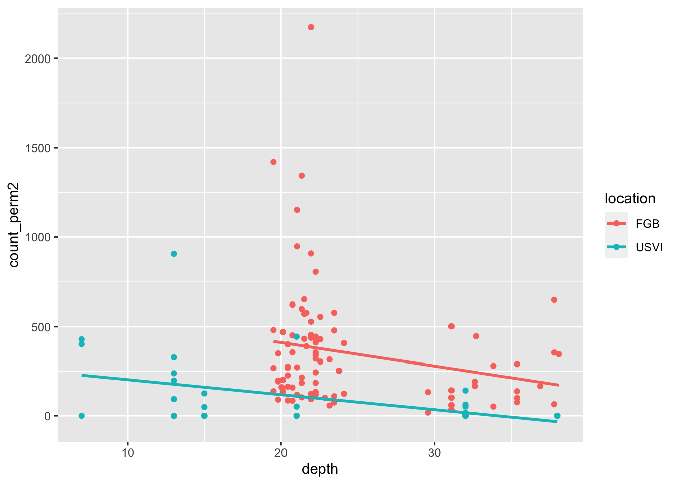
If we want to model count per square meter on depth in the FGB location, we can first try Poisson regression.
library(rstanarm)
barnacles <- filter(barnacles, location == "FGB")
model_barnacles <- stan_glm(count_perm2 ~ depth,
  data = barnacles,
  family = poisson,
  refresh = 0
)

pp_check(model_barnacles)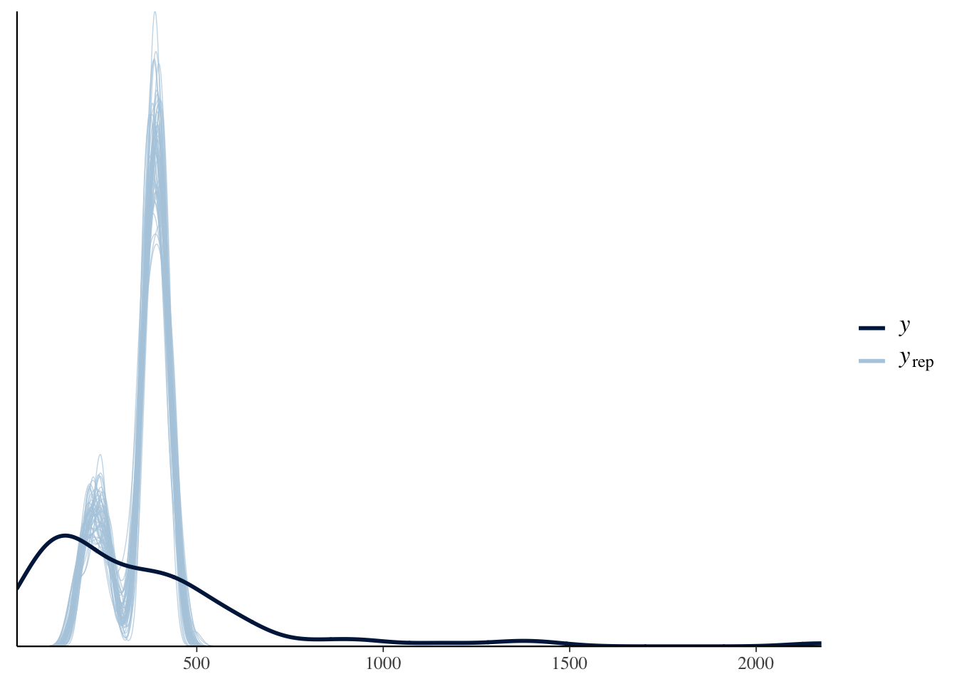
We see that this did not model the data well at all. Let’s switch to a negative binomial model:
model_barnacles <- stan_glm(count_perm2 ~ depth,
  data = barnacles,
  family = neg_binomial_2(),
  refresh = 0
)

bayesplot::pp_check(model_barnacles)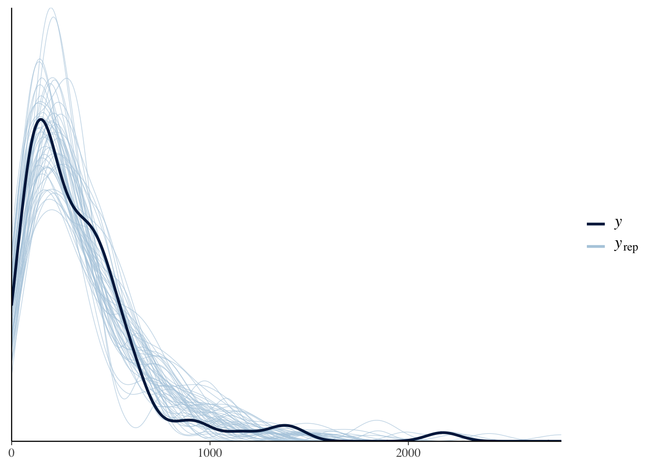
We see that the posterior predictive density aligns much better with the true data this way!
Now that we have seen that negative binomial regression can better model data that is overdispersed, we are ready to dive in to the model specifics a bit more. We model \(Y|_{X = x, \beta_0, \beta_1} \sim \mathrm{Negative Binommial}(r, \mu)\), where \(r\) is the (reciprocal) dispersion parameter and \(\mu\) is the mean. We assume a relationship between the mean count and the predictors is \(\log \mu = \beta_0 + \beta_1 x\). We choose normal priors for \(\beta_0\) and \(\beta_1\), and we choose an exponential prior for the dispersion parameter.
Find a reasonable value for the dispersion parameter from the barnacles data.
barnacles %>%
  group_by(cut(depth, 5)) %>%
  summarize(
    mu = mean(count_perm2),
    var = var(count_perm2),
    r = mu^2 / (var - mu)
  )
## # A tibble: 5 × 4
## `cut(depth, 5)` mu var r
## <fct> <dbl> <dbl> <dbl>
## 1 (19.5,23.2] 411. 139075. 1.22
## 2 (23.2,26.9] 290. 40023. 2.11
## 3 (26.9,30.7] 75.5 6612. 0.872
## 4 (30.7,34.4] 198. 26885. 1.47
## 5 (34.4,38.1] 243. 35878. 1.66We need that the variance is the mean plus the mean squared over r, which means that \(r = \frac{\mu^2}{\sigma^2 - \mu}\). The different cuts give values of \(r\) ranging from 0.872 to 2.11, so a reasonable estimate of \(r\) might be 1.4.
Let’s check that against the value that rstanarm found.
tidybayes::spread_draws(model_barnacles, `[\\(a-z].*`, regex = T) %>%
  janitor::clean_names() %>%
  summarize(r = HDInterval::hdi(reciprocal_dispersion))
## # A tibble: 2 × 1
## r
## <dbl>
## 1 1.19
## 2 2.07We see that the 95 percent credible interval for the dispersion parameter is \([1.20, 2.08]\), which isn’t that different than our crude estimate.
The interpretation of \(\beta_0\) and \(\beta_1\) are the same as in Poisson regression, so we do not review. Let’s end with an example.
Consider the bears_full data set in the bayeta package. This gives the number of offspring and mates of a group of bears in Canada, together with their statistics on rubbing on trees and posts. We wish to model the number of offspring on the other variables. This example will show some difficulties associated with the procedure. Let’s look at some plots:
bears <- bayeta::bears_full
ggplot(bears, aes(x = num_rubs, y = mates, color = sex)) +
  geom_point()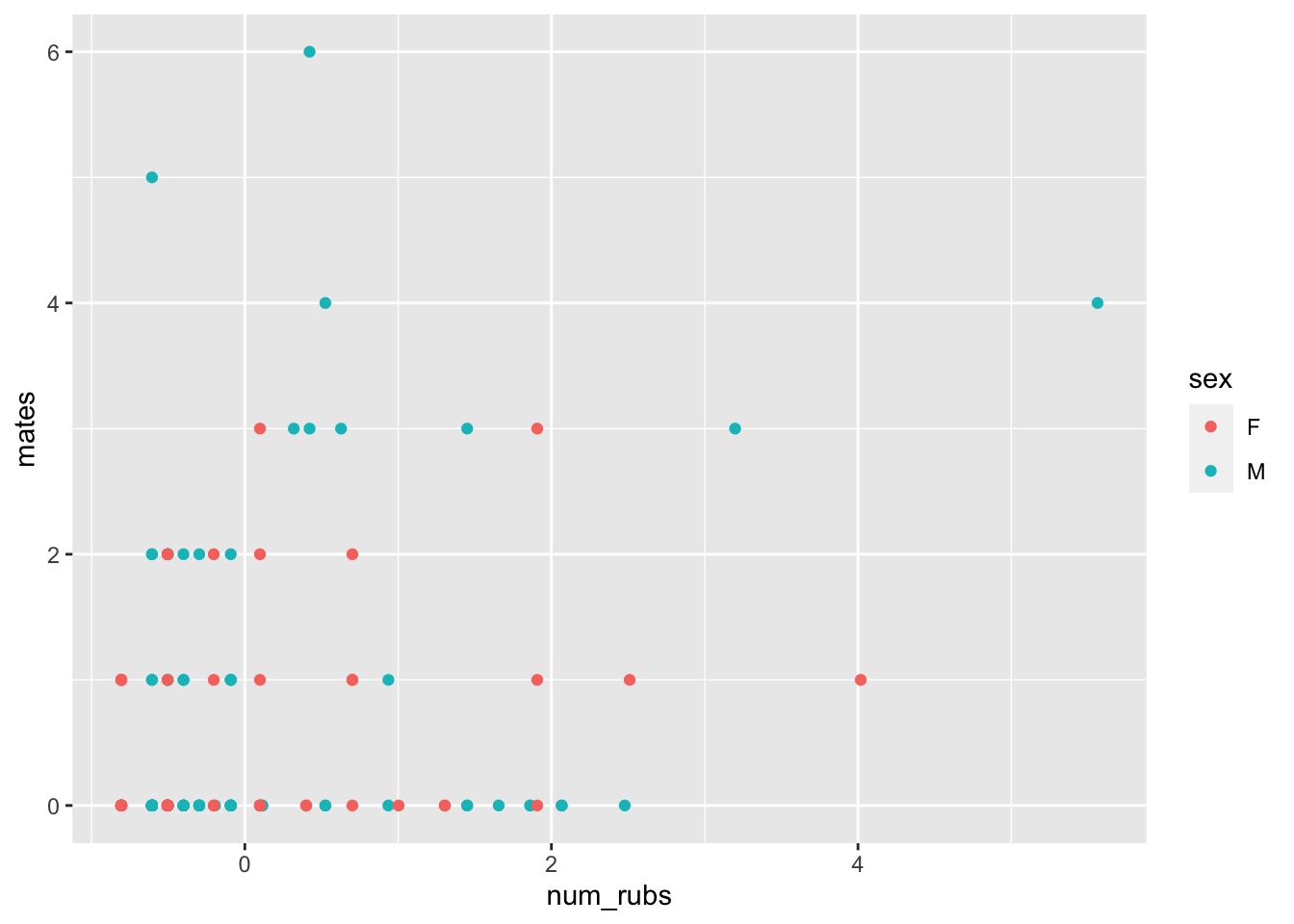
ggplot(bears, aes(x = num_occasion, y = mates, color = sex)) +
  geom_point()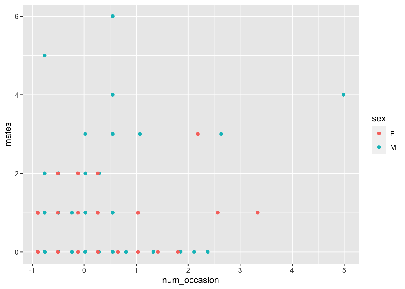
None of those are particularly compelling, but one thing to notice is that this is highly right skew. These variables have been standardized and even still we are getting values of 3, 4 and 5. That means those bears really liked to rub on posts and trees!
Let’s try Poisson regression on the number of offspring as described by the other variables.
offspring_model <- rstanarm::stan_glm(offspring ~ num_rubs + num_occasion + sex,
  data = bears,
  family = poisson,
  refresh = 0
)
broom.mixed::tidy(offspring_model)
## # A tibble: 4 × 3
## term estimate std.error
## <chr> <dbl> <dbl>
## 1 (Intercept) -0.324 0.155
## 2 num_rubs 0.168 0.165
## 3 num_occasion 0.181 0.174
## 4 sexM 0.156 0.196We see that all of the estimates (except intercept) are within 2 standard errors of zero, so would not be significant by frequentist techniques. Let’s check the posterior predictive density.
bayesplot::pp_check(offspring_model, plotfun = "ppc_hist")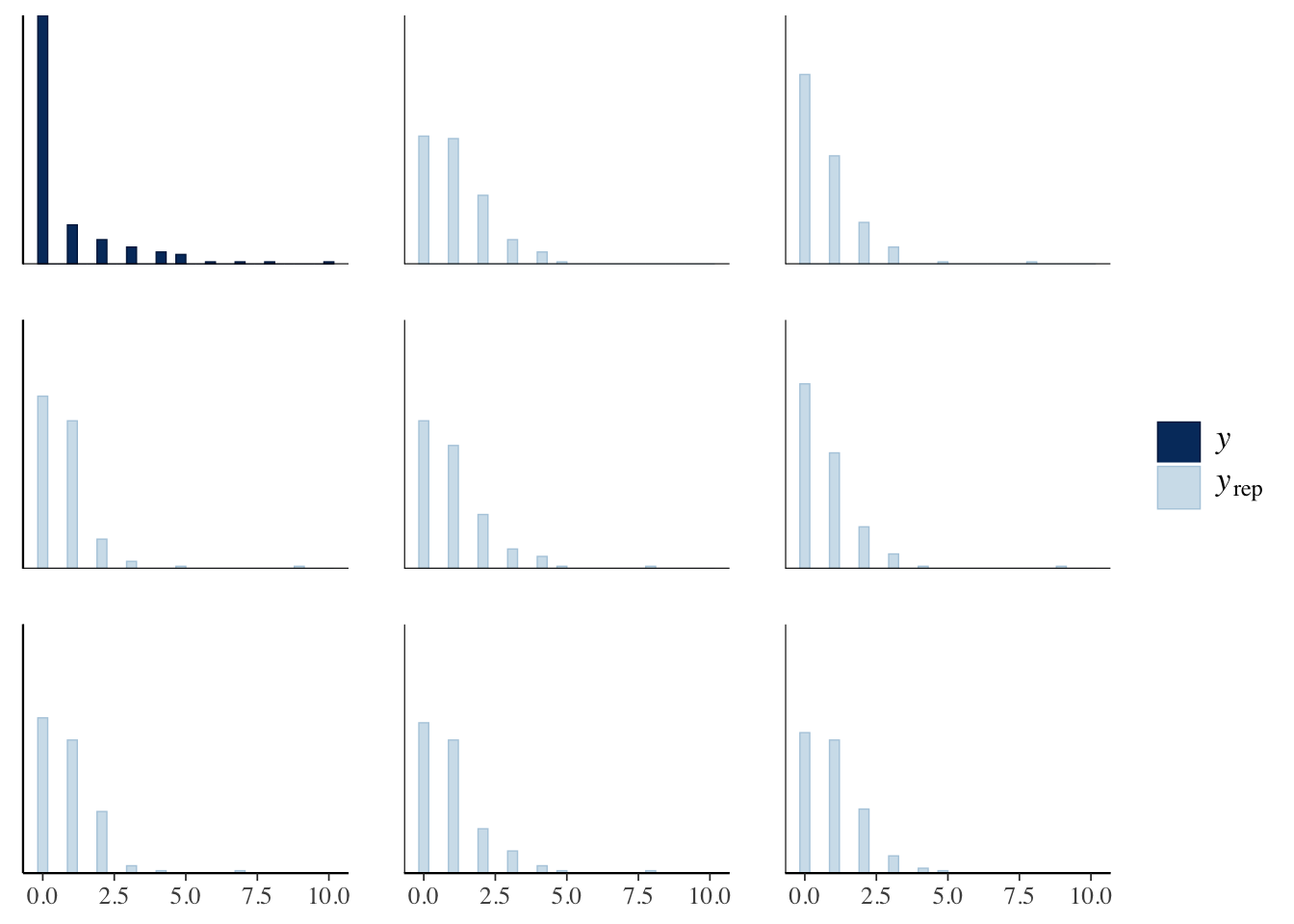
That looks OK maybe, except that we seem to be underestimating the probability of 0, and overestimating the other probabilities. Let’s check those more carefully, using code I copied.
prop_zero <- function(y) mean(y == 0)
pp_check(offspring_model, plotfun = "stat", stat = "prop_zero", binwidth = .005)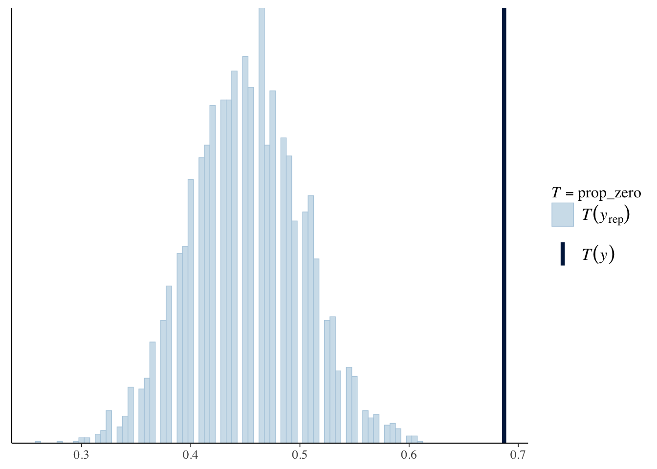
We see that the true proportion of zeros is near 0.7, which does not fall in the histogram of simulated proportions of zeros. Sometimes people will try a negative binomial model when the data is zero inflated in this way.
offspring_model_negbinom <- rstanarm::stan_glm(offspring ~ num_rubs + num_occasion + sex,
  data = bears,
  family = neg_binomial_2,
  refresh = 0
)
broom.mixed::tidy(offspring_model_negbinom)
## # A tibble: 4 × 3
## term estimate std.error
## <chr> <dbl> <dbl>
## 1 (Intercept) -0.329 0.319
## 2 num_rubs 0.244 0.393
## 3 num_occasion 0.229 0.373
## 4 sexM 0.199 0.393bayesplot::pp_check(offspring_model_negbinom, plotfun = "ppc_hist")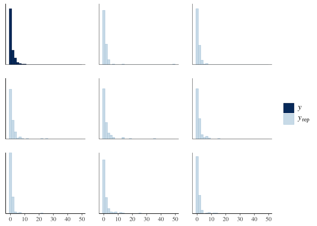
pp_check(offspring_model_negbinom, plotfun = "stat", stat = "prop_zero", binwidth = .005)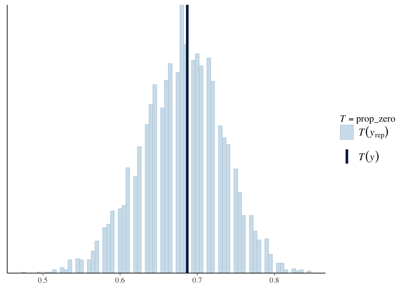
This seems to capture the zeros a lot better than our Poisson model, but also has other issues; for example, it is plausible to have up to 400 offspring for a single bear!
We can also check using cross validation whether the negative binomial or poisson model is better.
loo_nb <- loo(offspring_model_negbinom)
loo_pois <- loo(offspring_model)
loo_compare(loo_nb, loo_pois)
## elpd_diff se_diff
## offspring_model_negbinom 0.0 0.0
## offspring_model -57.2 16.7The negative binomial model is prefered, which isn’t surprising given that we see how much better it was with predicting \(y = 0\) offspring.
As one last comparison, we compare the model we built with a constant model.
bear_minimum <- rstanarm::stan_glm(offspring ~ 1,
  data = bears,
  family = neg_binomial_2(),
  refresh = 0
)

loo_constant <- rstanarm::loo(bear_minimum)

rstanarm::loo_compare(loo_constant, loo_nb)
## elpd_diff se_diff
## offspring_model_negbinom 0.0 0.0
## bear_minimum -0.5 1.9The model with three predictors does not have better out of bag expected log predictive density, at least not once we take into account the standard error.
pp_check(bear_minimum, plotfun = "stat", stat = "prop_zero", binwidth = .005)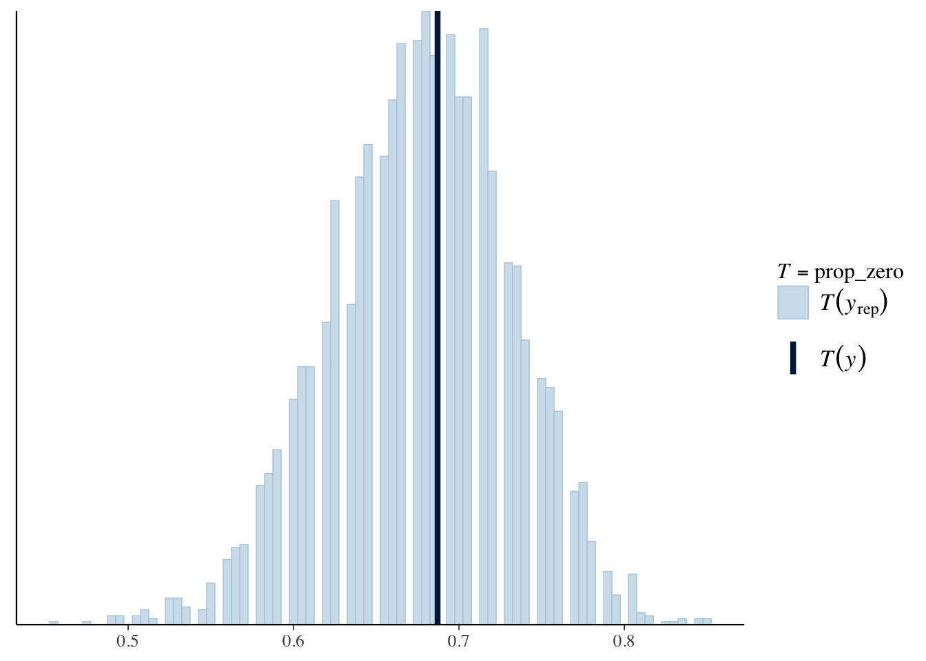
So far, we would be hard-pressed to recommend a model other than one that doesn’t depend on any of the predictors. Let’s consider just num_occasion:
occasion_model <- rstanarm::stan_glm(offspring ~ num_occasion,
  data = bears,
  family = neg_binomial_2(),
  refresh = 0
)
broom.mixed::tidy(occasion_model)
## # A tibble: 2 × 3
## term estimate std.error
## <chr> <dbl> <dbl>
## 1 (Intercept) -0.212 0.184
## 2 num_occasion 0.430 0.191loo_occasion <- loo(occasion_model)
loo_compare(loo_occasion, loo_constant)## elpd_diff se_diff
## occasion_model 0.0 0.0
## bear_minimum -1.9 2.0While the model on num_occasion doesn’t bear bear_minimum by 2 standard errors, it does beat it by one standard error, which is a different rule of thumb that one sees.
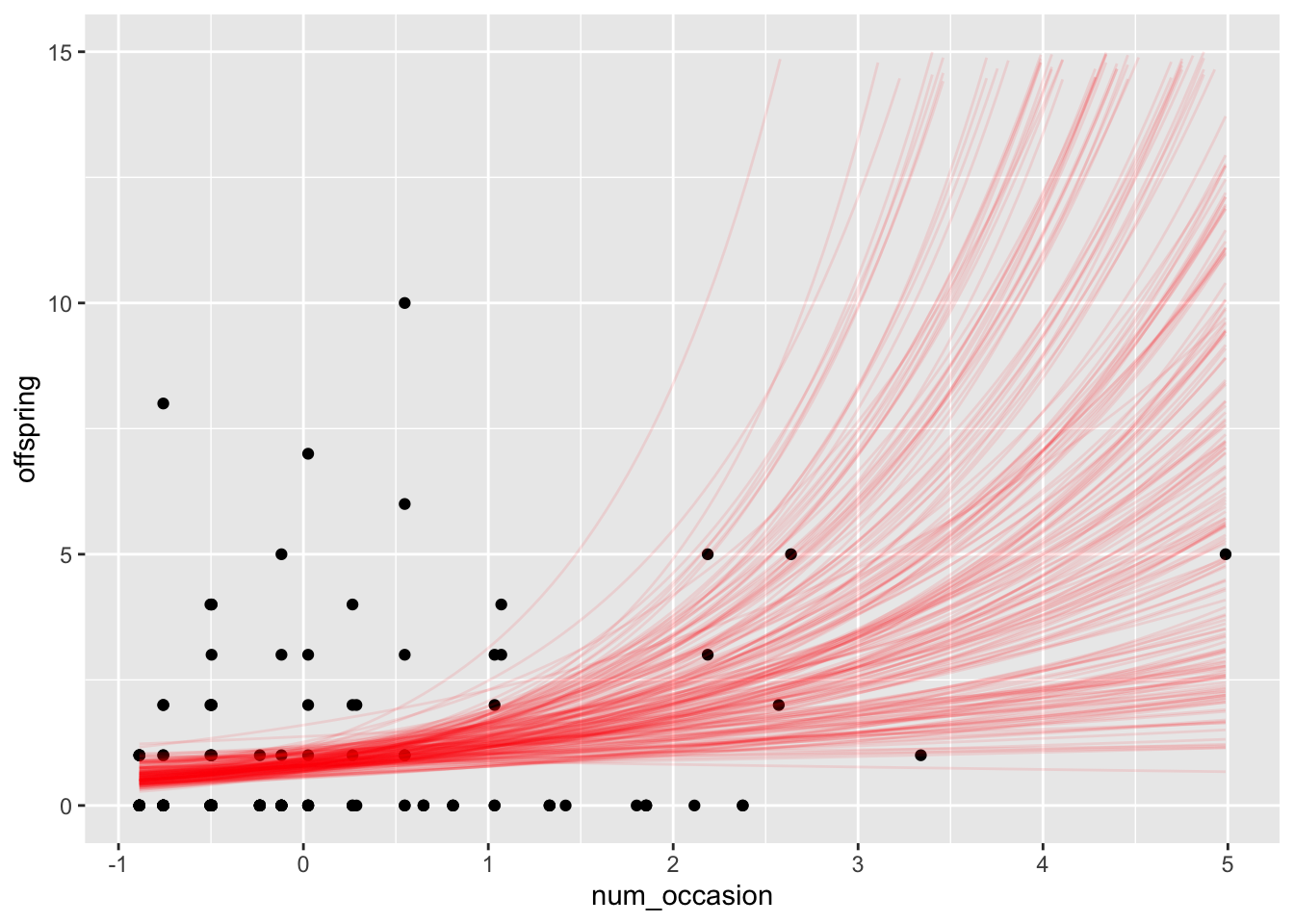
bear_draws <- tidybayes::spread_draws(occasion_model, `[\\(a-z].*`, regex = T, ndraws = 200) %>%
  janitor::clean_names()

funcs <- lapply(1:200, function(i) {
  geom_function(
    fun = function(x) exp(bear_draws$intercept[i] + x * bear_draws$num_occasion[i]),
    alpha = 0.1,
    color = "red"
  )
})

ggplot(bears, aes(x = num_occasion, y = offspring)) +
  geom_point() +
  funcs +
  scale_y_continuous(limits = c(0, 15))