Chapter 4 Extending the Normal Regression Model
In this chapter, we consider what happens in the usual case when we have more than one predictor variable.
4.1 A categorical predictor
Following the example in the text, we consider the weather_WU data set in the bayesrules package. This data gives the temperature at 9 AM and at 3 PM in two Australian cities. We are interested in modeling the temperature at 3 PM based on the same day temperature at 9 AM.
ww <- bayesrules::weather_WU
head(ww)
## # A tibble: 6 × 22
## location mintemp maxtemp rainfall windgustdir windgustspeed winddir9am
## <fct> <dbl> <dbl> <dbl> <ord> <dbl> <ord>
## 1 Uluru 12.3 30.1 0 ENE 39 E
## 2 Uluru 20.5 35.9 5 SSE 52 SE
## 3 Uluru 15.8 41.4 0 NNW 50 SSE
## 4 Uluru 18.3 36 0 SE 57 E
## 5 Uluru 28.9 44.8 0 ENE 44 ESE
## 6 Uluru 18.1 35.9 0 ESE 35 ESE
## # … with 15 more variables: winddir3pm <ord>, windspeed9am <dbl>,
## # windspeed3pm <dbl>, humidity9am <int>, humidity3pm <int>,
## # pressure9am <dbl>, pressure3pm <dbl>, temp9am <dbl>, temp3pm <dbl>,
## # raintoday <fct>, risk_mm <dbl>, raintomorrow <fct>, year <dbl>,
## # month <dbl>, day_of_year <dbl>One thing we might be worried about is that this is data collected over time. If we are planning on using this to predict 3 PM temperatures in the future, it would be worth knowing whether the error in our model is correlated with time. That is, after we have accounted for the other variables in our model, is the fact that the 3 PM temperature is higher [resp lower] than predicted correlated with the 3 PM temperature of the next day being higher [resp lower] than predicted. However, in this case we are ignoring that. We are simply taking a random sample of size 200 over the last 5 or so years, and trying to model the 3 PM temperature based on the 9 AM temperature. This may seem a bit like an academic exercise, because it is hard to think of what we would use this model for, other than to predict 3 PM temperatures in the future, based on 9 AM temperatures.
As a warm-up, let’s see how to model the 9 AM temperatures on the single categorical predictor location. We start with a density plot of the temperature in both locations, using ggridges.
library(ggridges)
ggplot(ww, aes(x = temp9am, y = location)) +
  geom_point() +
  geom_density_ridges(alpha = .6, fill = "lightblue") +
  theme_minimal()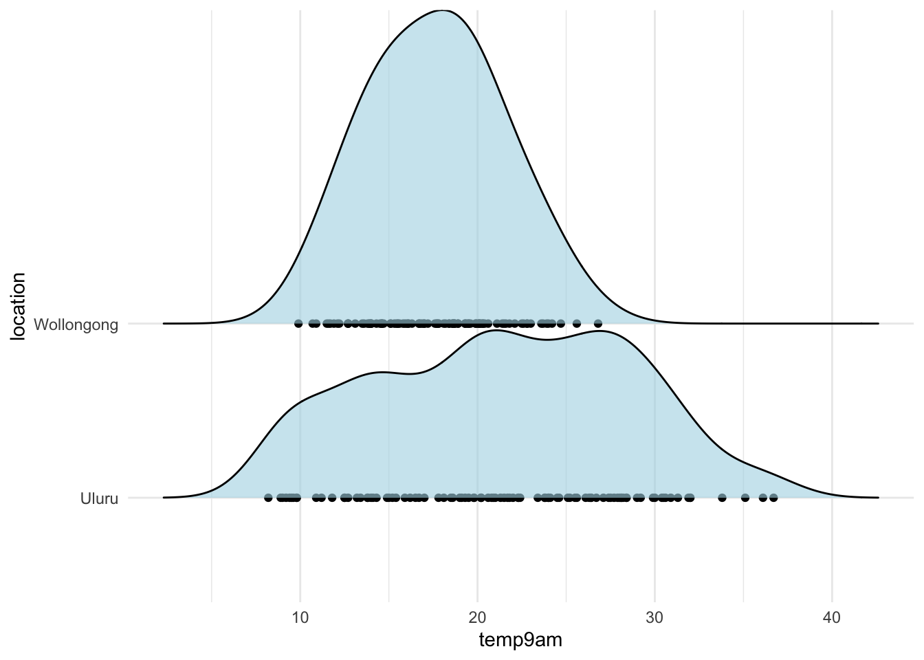
There are several ways to conceptualize a single categorical predictor. Let’s see how stan_glm does it.
single_cat <- rstanarm::stan_glm(temp9am ~ location,
  data = ww,
  refresh = 0
)
tidybayes::get_variables(single_cat)
## [1] "(Intercept)" "locationWollongong" "sigma"
## [4] "accept_stat__" "stepsize__" "treedepth__"
## [7] "n_leapfrog__" "divergent__" "energy__"We see there are 3 variables that are of interest: the intercept, locationWollongong, and sigma. Let’s pull them out.
tidybayes::spread_draws(single_cat, `[\\(sl].*`, regex = T) %>%
  summarize(across(.fns = mean))
## # A tibble: 1 × 7
## .chain .iteration .draw `(Intercept)` locationWollongong sigma
## <dbl> <dbl> <dbl> <dbl> <dbl> <dbl>
## 1 2.5 500. 2000. 21.5 -3.82 5.78
## # … with 1 more variable: stepsize__ <dbl>We see that a typical value for the intercept is 21.4, and for Wollongong is -3.81, and for sigma is 5.79. That roughly corresponds to the mean temperature for Uluru, and the difference between Uluru and Wollongong. The standard deviation is neither. The standard deviation corresponds to approximately the standard deviation of all of the values.
ww %>%
  group_by(location) %>%
  summarize(
    mu = mean(temp9am),
    sd = sd(temp9am)
  )
## # A tibble: 2 × 3
## location mu sd
## <fct> <dbl> <dbl>
## 1 Uluru 21.4 7.22
## 2 Wollongong 17.6 3.76sd(ww$temp9am)## [1] 6.051522In order to state our model, we create an indicator variable \(x\) that is 1 when the location is Wollongong and 0 when the location is Uluru. We could add it to our data like this, but we don’t have to.
ww %>%
  mutate(x = as.integer(stringr::str_detect(location, "Woll"))) %>%
  select(location, temp9am, x) %>%
  sample_n(10) # this is just to see a few x values that are 0 and that are 1
## # A tibble: 10 × 3
## location temp9am x
## <fct> <dbl> <int>
## 1 Wollongong 11.7 1
## 2 Uluru 28.1 0
## 3 Wollongong 20 1
## 4 Wollongong 17.8 1
## 5 Uluru 22.3 0
## 6 Wollongong 13.5 1
## 7 Wollongong 17.8 1
## 8 Uluru 14 0
## 9 Uluru 19.3 0
## 10 Uluru 16.2 0Our model is \(Y = \beta_0 + \beta_1 x + \epsilon\), where \(\epsilon\) is normally distributed with mean \(\sigma\). We have the same assumptions as before regarding idependence and normal distribution of errors with the same distribution across all levels of the predictor(s). If you think about this model a bit, you will see that it is equivalent to finding \(\beta_0\), \(\beta_1\) and \(\sigma\) so that the 9 AM temperature in Uluru is normal with mean \(\beta_0\) and sd \(\sigma\), and so that the 9 AM temperature in Wollongong is normal with mean \(\beta_0 + \beta_1\) and sd \(\sigma\).
Let’s check the posterior predictive distribution against the actual data, and we will see that this model may not be perfect because the standard deviation may not really be the same in both groups.
library(tidybayes)
spread_draws(single_cat, `[\\(sl].*`, regex = T) %>%
  janitor::clean_names() %>%
  mutate(
    uluru_val = rnorm(n(), intercept, sigma),
    wollongong_val = rnorm(n(), intercept + location_wollongong, sigma)
  ) %>%
  ggplot(aes(x = uluru_val)) +
  geom_density(color = "lightblue") +
  geom_density(data = filter(ww, location == "Uluru"), mapping = aes(x = temp9am))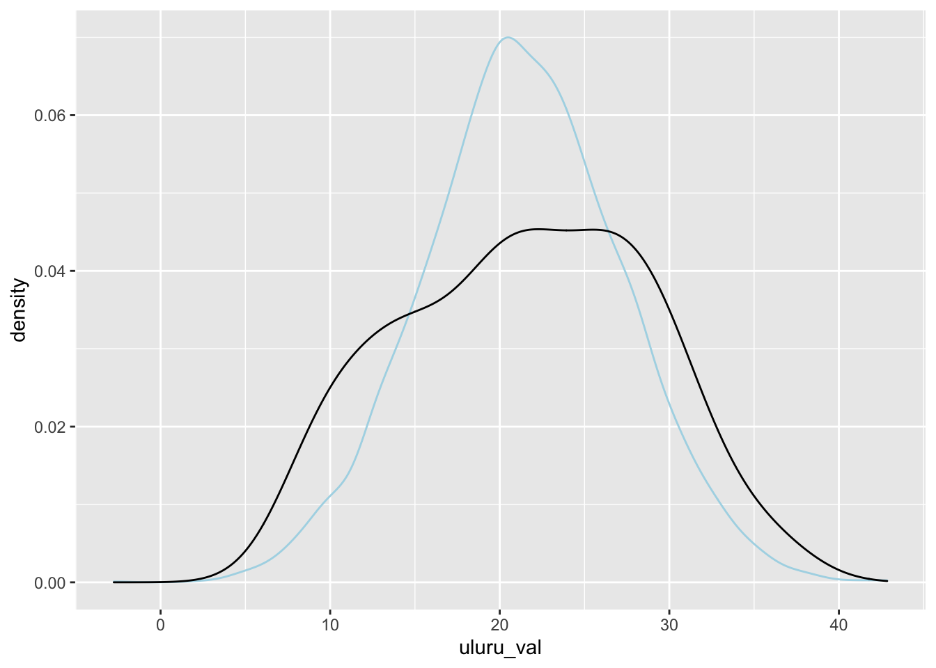
This model is not the best for this data, but it was only meant to illustrate what happens when you have a single categorical predictor. If you have more levels in your categorical predictor, then you would create more indicator variables. We do not go into the details.
Now, let’s model the 3 PM temperature on the 9 AM temperature and see what we get. We set prior_PD = TRUE so that we can understand what priors were chosen automatically for us.
library(rstanarm)
model_9am <- rstanarm::stan_glm(temp3pm ~ temp9am + location,
  data = ww,
  refresh = 0
)
We check some diagnostics:
library(bayesplot)
mcmc_acf(model_9am)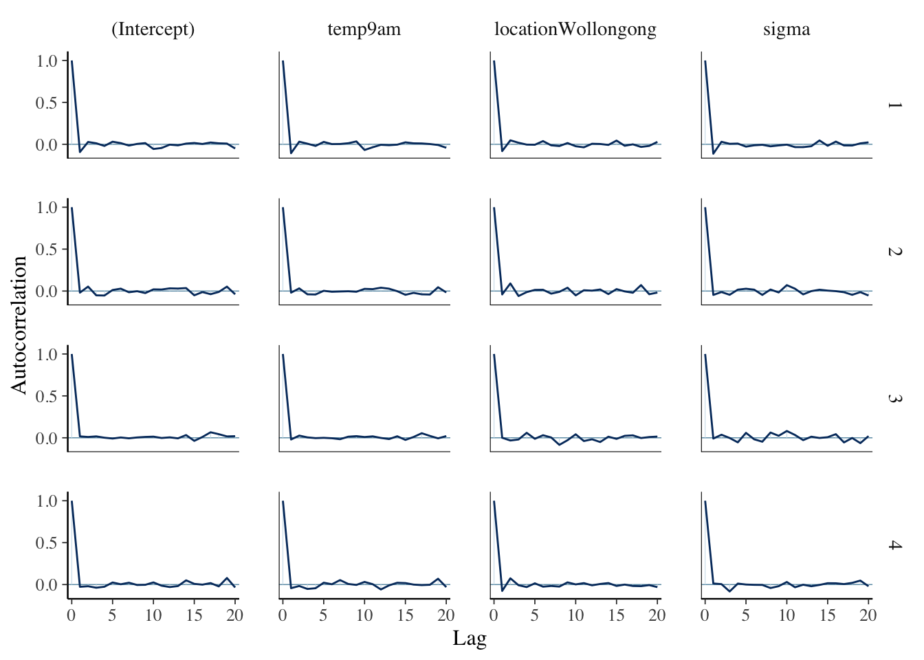
mcmc_dens_chains(model_9am)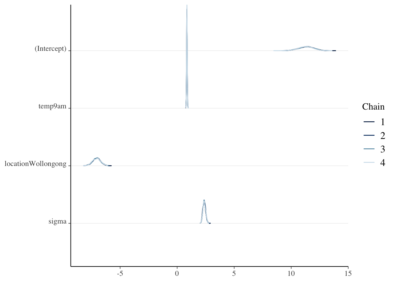
We probably should have visualized this!
ggplot(ww, aes(x = temp9am, y = temp3pm, color = location)) +
  geom_point() +
  geom_smooth(method = "lm", se = F)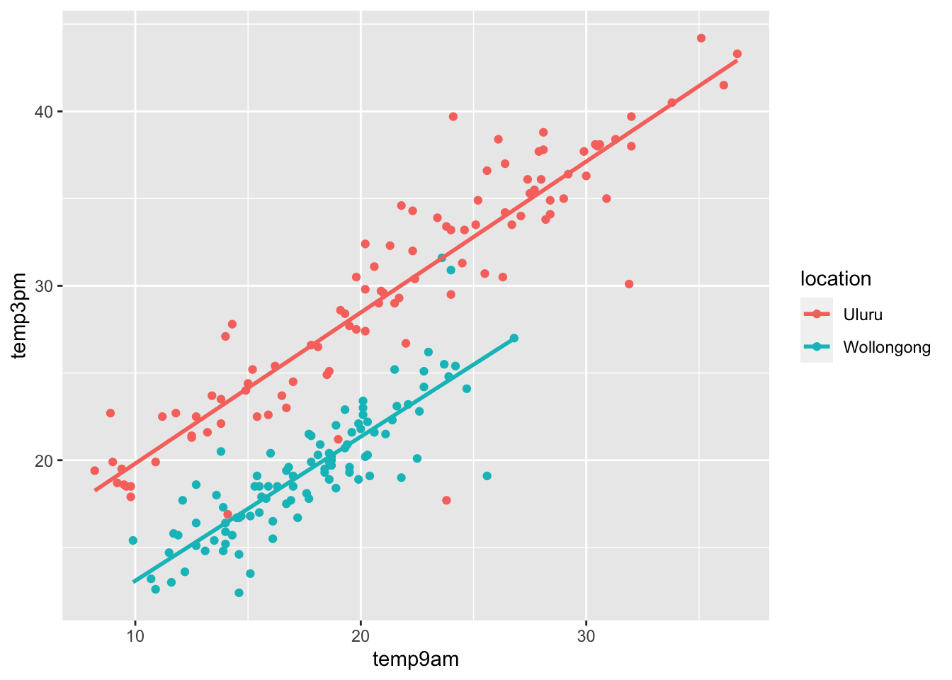
The model that we chose was \(Y = \beta_0 + \beta_1 \mathrm{temp9am} + \beta_2 x + \epsilon\), where \(x\) is as above and is 1 when the location is Wollongong and 0 when the location is Uluru. We are modeling the slope as the same in both locations, meaning that we believe that each degree higher in the morning corresponds to the same increase in the afternoon in both locations. Since the two lines on the plot are parallel, that seems reasonable in this case. We are also assuming that the errors are normal and the standard deviation is about the same in both groups. That may not be completely reasonable, because Uluru has some pretty far outliers.
We can look at a histogram of the residuals to see whether things look normal.
hist(residuals(model_9am))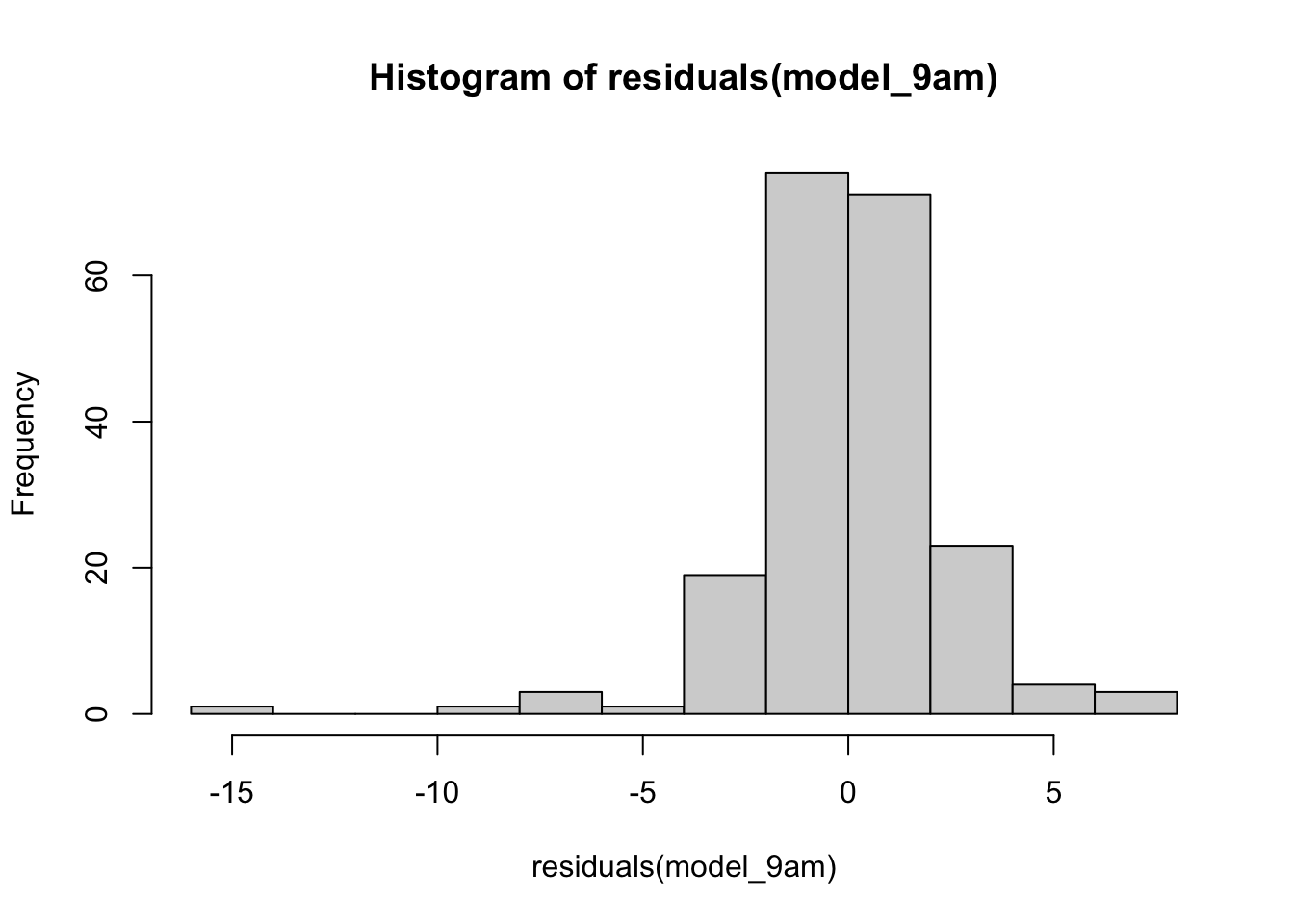
Normally distributed would not be my first thought looking at that!
Let’s also see what the priors were, and how they compare to the posteriors:
rstanarm::posterior_vs_prior(model_9am)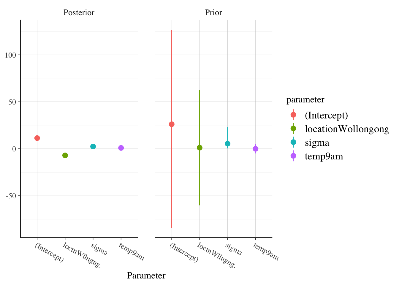
Note that we can’t even see the variation in the posterior draws, because the variation in the prior draws are so much bigger. This inidcates to me that the priors were sufficiently vague and reasonable. If we want to look more closely at sigma, for example, then we can use:
posterior_vs_prior(model_9am, pars = "sigma")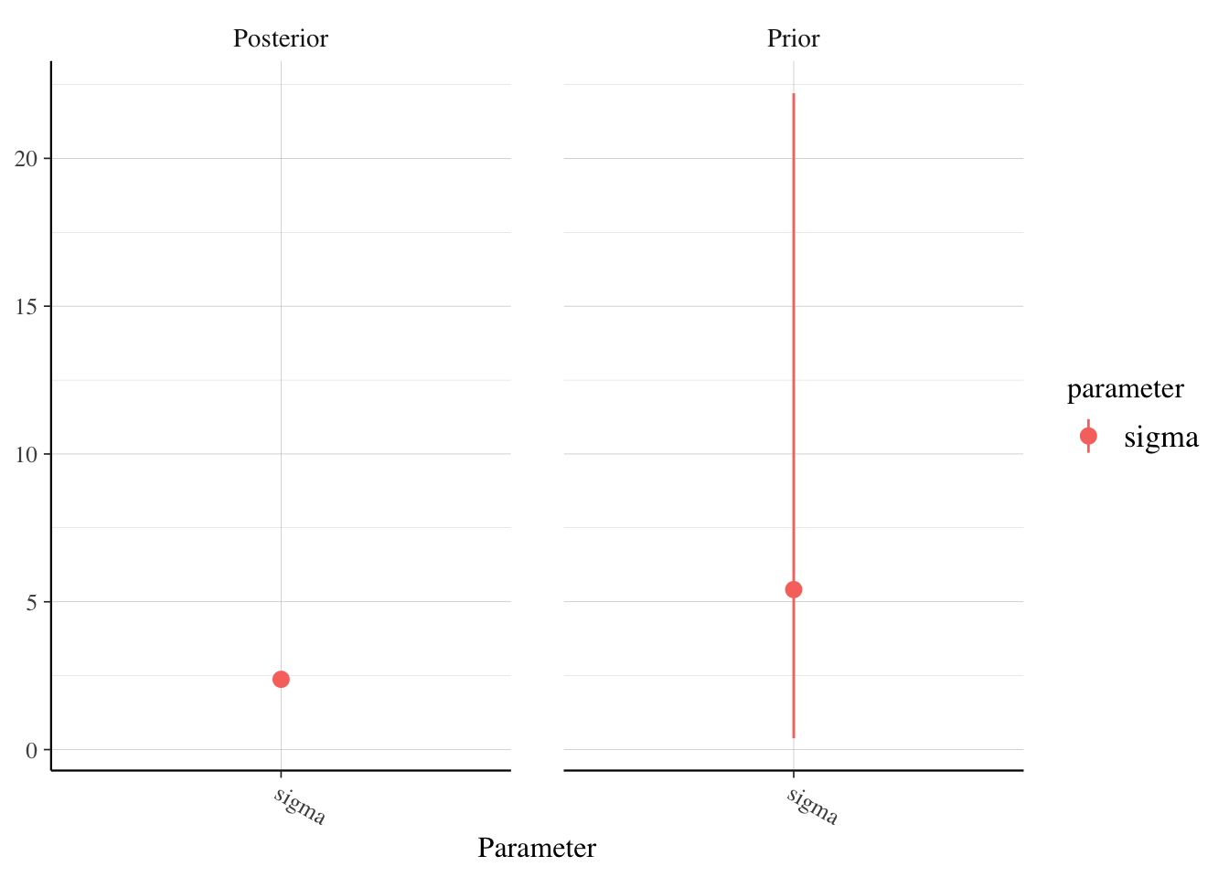
Let’s write out the entire model, including the priors. We have \(Y = \beta_0 + \beta_1 \mathrm{temp9am} + \beta_2 x + \epsilon\), where \(x\) is as above and is 1 when the location is Wollongong and 0 when the location is Uluru. The priors chosen were: \(\beta_0 \sim N(25, \sigma = 19)\) (after predictors were centered), \(\beta_1 \sim N(0, 3.11)\) and \(\beta_2 \sim N(0, 37.52)\), and \(\sigma \sim Exp(0.13)\).
Find a 95 percent posterior prediction interval for the 3 PM temperature in Wollongong if the 9 AM temperature is 20.
We start by creating a data frame of draws:
tidybayes::spread_draws(model_9am, `[\\(a-z].*`, regex = T) %>%
  janitor::clean_names() %>%
  mutate(val = rnorm(n(), intercept + location_wollongong + temp9am * 20, sigma)) %>%
  select(val) %>%
  summarize(HDInterval::hdi(val))
## # A tibble: 2 × 1
## `HDInterval::hdi(val)`
## <dbl>
## 1 16.6
## 2 26.0Perform cross-validation to check the achieved coverage of a 66 percent posterior prediction interval.
We do this in two different ways. First, using the function from bayesrules.
cv_model <- bayesrules::prediction_summary_cv(data = ww, model = model_9am, k = 10, prob_inner = .66, prob_outer = .95)
cv_model$cv
## mae mae_scaled within_66 within_95
## 1 1.060981 0.4436716 0.77 0.96We get 79 percent. That means that we can expect about 79 percent of future values to be in the 66 percent posterior prediction interval.
Next, we show how to do leave-one-out cross-validation. In this version, we build the model on all points except for one, and see whether the one left out falls in the prediction interval. We repeat for all observations.
library(future.apply)
plan("multisession")
cv_loo <- future.apply::future_sapply(1:nrow(ww), function(x) {
  ww_short <- ww[-x, ]
  model_9am <- rstanarm::stan_glm(temp3pm ~ temp9am + location,
    data = ww_short,
    refresh = 0
  )
  is_woll <- stringr::str_detect(ww$location[x], "ollon")
  hdi <- tidybayes::spread_draws(model_9am, `[\\(a-z].*`, regex = T) %>%
    janitor::clean_names() %>%
    mutate(val = rnorm(n(), intercept + location_wollongong * is_woll + temp9am * ww$temp9am[x], sigma)) %>%
    select(val) %>%
    summarize(hdi = HDInterval::hdi(val, credMass = 0.66))
  ww$temp3pm[x] < hdi$hdi[2] && ww$temp3pm[x] > hdi$hdi[1]
}, future.seed = TRUE)
plan("sequential")
mean(cv_loo)
## [1] 0.76This says we have about 76 percent coverage, which means that our LOOCV estimate would be that this posterior predictive interval is a 76 percent posterior prediction interval, and not a 66 percent ppi. A more sophisticated approach (especially if we are using this to compare two models) would be to build the model after leaving out a single variable and look at the likelihood (under the posterior) of the left-out data point. The model that has the higher posterior probability for the left out data points would be a better choice. We will come back to this point later in the notes.
In the example that we did above, the slope was assumed to be the same for the two cities. That means that a one degree increase in 9 AM temperature would lead to the same expected increase in 3 PM temperature in each city. Sometimes, that is not the case though. Let’s consider the 3 PM temperature as described by the 9 AM humidity.
ggplot(ww, aes(x = humidity9am, y = temp3pm, color = location)) +
  geom_point() +
  geom_smooth(method = "lm")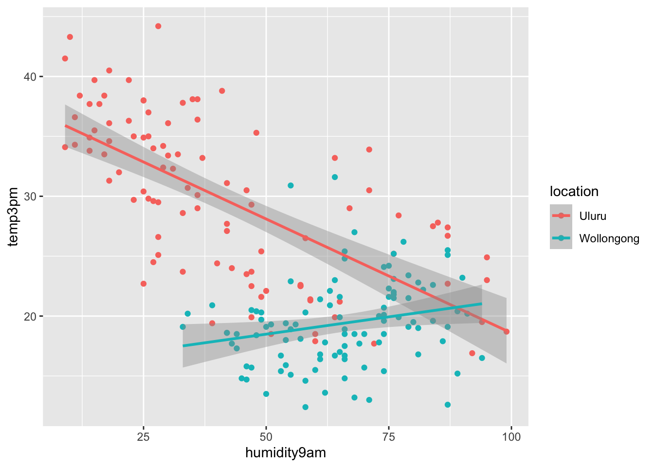
It appears that higher humidity is associated with lower temps in Uluru, and with warmer temps in Wollongong. In this case, it would be unwise to assume that the slope of each line is equal! We need to add an interaction term. Recall that the location variable was coded by adding a 0/1 variable that was 0 when the location is Uluru and 1 when the location is Wollongong, and including that in the regression model. The interaction term is created by multiplying the 0/1 variable created in the previous sentence by the humidity variable and including that in the model. Like this:
ww %>%
  select(humidity9am, temp3pm, location) %>% # just to make the df simpler
  mutate(is_woll = as.integer(stringr::str_detect(location, "ollon"))) %>%
  mutate(interaction = is_woll * humidity9am) %>%
  sample_n(6)
## # A tibble: 6 × 5
## humidity9am temp3pm location is_woll interaction
## <int> <dbl> <fct> <int> <int>
## 1 20 32 Uluru 0 0
## 2 31 32.3 Uluru 0 0
## 3 94 16.5 Wollongong 1 94
## 4 14 33.8 Uluru 0 0
## 5 50 22.1 Uluru 0 0
## 6 51 18.5 Uluru 0 0Let’s create that data frame and store it for future reference.
ww_narrow <- ww %>%
  select(humidity9am, temp3pm, location) %>% # just to make the df simpler
  mutate(is_woll = as.integer(stringr::str_detect(location, "ollon"))) %>%
  mutate(interaction = is_woll * humidity9am)
In order to indicate to stan_glm that we want to allow different slopes for the two locations, we use the following.
model_interaction_weather <- stan_glm(temp3pm ~ humidity9am + location + location:humidity9am,
  data = ww,
  refresh = 0
)

prior_summary(model_interaction_weather)
## Priors for model 'model_interaction_weather'
## ------
## Intercept (after predictors centered)
## Specified prior:
## ~ normal(location = 25, scale = 2.5)
## Adjusted prior:
## ~ normal(location = 25, scale = 19)
##
## Coefficients
## Specified prior:
## ~ normal(location = [0,0,0], scale = [2.5,2.5,2.5])
## Adjusted prior:
## ~ normal(location = [0,0,0], scale = [ 0.82,37.52, 0.55])
##
## Auxiliary (sigma)
## Specified prior:
## ~ exponential(rate = 1)
## Adjusted prior:
## ~ exponential(rate = 0.13)
## ------
## See help('prior_summary.stanreg') for more detailsLet’s check some diagnostics.
bayesplot::rhat(model_interaction_weather)## (Intercept) humidity9am
## 1.000019 1.000156
## locationWollongong humidity9am:locationWollongong
## 1.001357 1.001153
## sigma
## 1.000463mcmc_dens_chains(model_interaction_weather, regex_pars = "humi")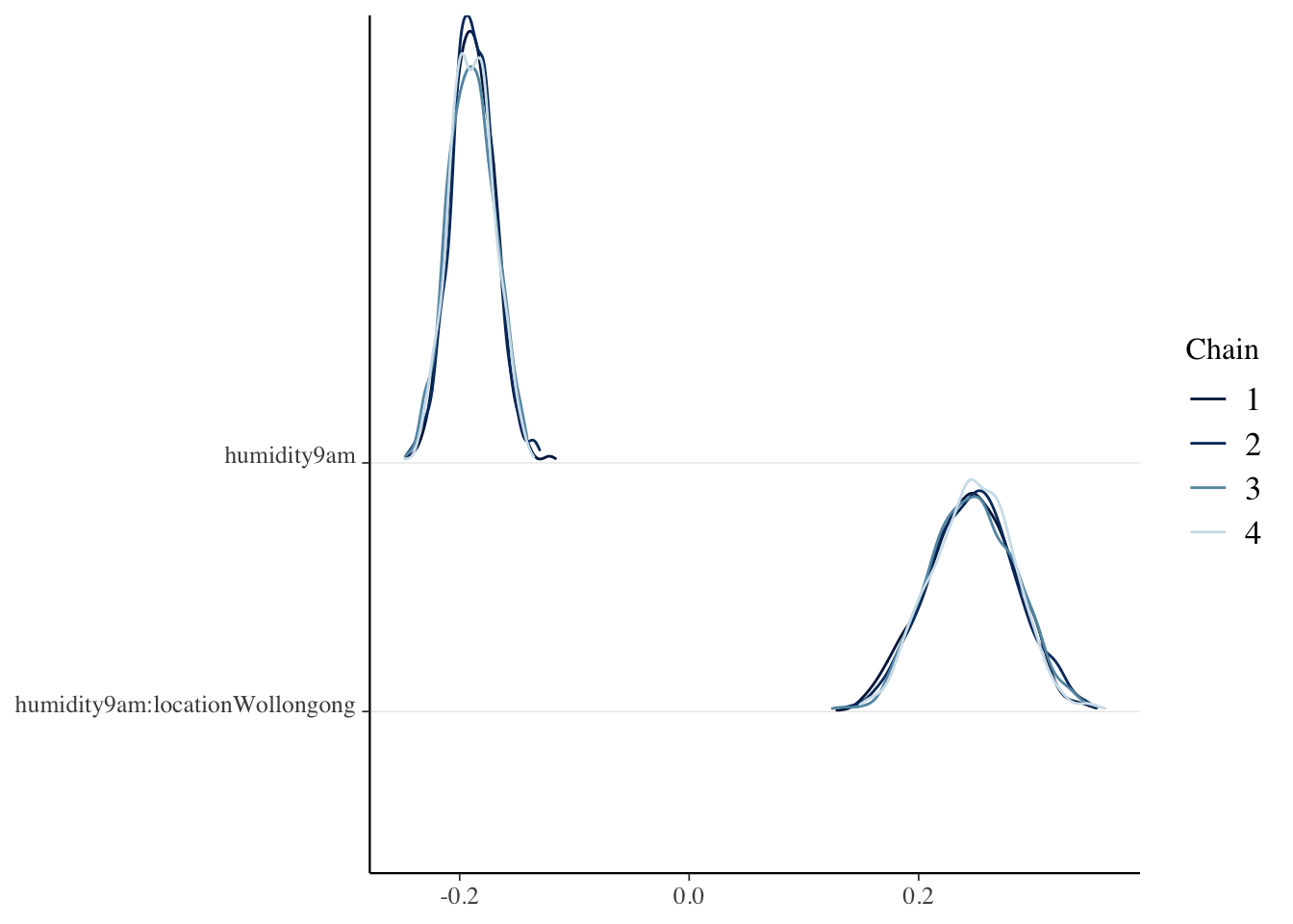
What are the median values for the coefficients, and what is the model?
summary(model_interaction_weather)##
## Model Info:
## function: stan_glm
## family: gaussian [identity]
## formula: temp3pm ~ humidity9am + location + location:humidity9am
## algorithm: sampling
## sample: 4000 (posterior sample size)
## priors: see help('prior_summary')
## observations: 200
## predictors: 4
##
## Estimates:
## mean sd 10% 50% 90%
## (Intercept) 37.6 0.9 36.4 37.6 38.7
## humidity9am -0.2 0.0 -0.2 -0.2 -0.2
## locationWollongong -21.9 2.4 -25.0 -22.0 -18.9
## humidity9am:locationWollongong 0.2 0.0 0.2 0.2 0.3
## sigma 4.5 0.2 4.2 4.5 4.8
##
## Fit Diagnostics:
## mean sd 10% 50% 90%
## mean_PPD 24.6 0.4 24.0 24.6 25.1
##
## The mean_ppd is the sample average posterior predictive distribution of the outcome variable (for details see help('summary.stanreg')).
##
## MCMC diagnostics
## mcse Rhat n_eff
## (Intercept) 0.0 1.0 2356
## humidity9am 0.0 1.0 2230
## locationWollongong 0.1 1.0 1980
## humidity9am:locationWollongong 0.0 1.0 1819
## sigma 0.0 1.0 3362
## mean_PPD 0.0 1.0 3269
## log-posterior 0.0 1.0 1773
##
## For each parameter, mcse is Monte Carlo standard error, n_eff is a crude measure of effective sample size, and Rhat is the potential scale reduction factor on split chains (at convergence Rhat=1).Our model is \(Y = \beta_0 + \beta_1 \mathrm{humidity9am} + \beta_2 x + \beta_3 w + \epsilon\), where \(x\) is equal to 1 when the location is Wollongong and 0 otherwise, \(w\) is equal to the humidity at 9 AM when the location is Wollongong and 0 otherwise, and \(\epsilon\) is independent and normally distributed with mean 0 and standard deviation \(\sigma\).
Our point estimates for the parameters would be \(\beta_0 = 37.6\), \(\beta_1 = -0.2\), \(\beta_3 = -21.9\), \(\beta_3 = 0.2\), and \(\sigma = 4.5\). As a specific example, let’s find the expected value of the temperature at 3 PM in Wollongong if the humidity at 9 AM is 60 percent. We would get (we should use more significant digits):
37.6 - 0.2 * 60 - 21.9 + 0.2 * 60## [1] 15.7Note that for Wollongong, the slope becomes \((\beta_1 + \beta_3)\), and the intercept is \(\beta_0 + \beta_2\). You might reasonably wonder why we didn’t just build two separate models for Wollongong and Ulrulu. The only difference here is that we are assuming that \(\sigma\) is the same across both models. If that is not the case, then we should build two separate models.
Use cross-validation to estimate the coverage of a 50 percent posterior prediction interval for the high temperature at 3 PM.
We again do it two ways.
cv_model <- bayesrules::prediction_summary_cv(data = ww, model = model_interaction_weather, k = 10)
cv_model$cv
## mae mae_scaled within_50 within_95
## 1 3.118694 0.6933564 0.54 0.95We see that this model is behaving as designed, as far as 50 percent and 95 percent prediction intervals go.
Again, it is instructive to do this by hand using LOOCV, though only grad students are responsible for being able to reproduce this, Since we already have the variables that match the coefficients in ww_narrow, we can most easily use that.
x <- 1
hdi <- spread_draws(model_interaction_weather, `[\\(a-z].*`, regex = T) %>%
  select(!matches("_$")) %>%
  janitor::clean_names() %>%
  mutate(post = rnorm(
    n(), intercept + humidity9am * ww_narrow$humidity9am[x] +
      location_wollongong * ww_narrow$is_woll[x] +
      humidity9am_location_wollongong * ww_narrow$interaction[x],
    sigma
  )) %>%
  select(post) %>%
  summarize(val = HDInterval::hdi(post, credMass = .5))
ww_narrow$temp3pm[x] < hdi$val[2] && ww_narrow$temp3pm[x] > hdi$val[1]
## [1] TRUElibrary(future.apply)
plan("multisession")
tf <- future_sapply(1:200, function(x) {
hdi <- spread_draws(model_interaction_weather, `[\\(a-z].*`, regex = T) %>%
select(!matches("_$")) %>%
janitor::clean_names() %>%
mutate(post = rnorm(
n(), intercept + humidity9am * ww_narrow$humidity9am[x] +
location_wollongong * ww_narrow$is_woll[x] +
humidity9am_location_wollongong * ww_narrow$interaction[x],
sigma
)) %>%
select(post) %>%
summarize(val = HDInterval::hdi(post, credMass = .5))
ww_narrow$temp3pm[x] < hdi$val[2] && ww_narrow$temp3pm[x] > hdi$val[1]
}, future.seed = TRUE)
mean(tf)## [1] 0.545plan("sequential")4.2 Adding more predictors
Continuing with the weather example, we can predict the 3 PM weather in the two cities based on all of the weather information available at 9 AM. Let’s pull out the interesting variables first.
ww_mult <- select(ww, matches("9am$|^temp|location"))
head(ww_mult)
## # A tibble: 6 × 7
## location winddir9am windspeed9am humidity9am pressure9am temp9am
## <fct> <ord> <dbl> <int> <dbl> <dbl>
## 1 Uluru E 20 23 1023. 20.9
## 2 Uluru SE 9 71 1013. 23.4
## 3 Uluru SSE 7 15 1012. 24.1
## 4 Uluru E 28 29 1016 26.4
## 5 Uluru ESE 24 10 1010. 36.7
## 6 Uluru ESE 22 32 1012. 25.1
## # … with 1 more variable: temp3pm <dbl>We see there are 4 continuous predictors and 2 categorical predictors for the 3 PM temperature. But wait! wind9am isn’t categorical, but an ordered factor, so an order of the wind directions is assumed. Independent of whether that is a good idea, we don’t know what would change if we had an ordered factor in a regression model, so our choices are to change it to a factor or to not use it… Let’s remove it.
ww_mult <- select(ww_mult, -matches("windd"))
mult_model <- rstanarm::stan_glm(temp3pm ~ ., data = ww_mult, refresh = 0)
summary(mult_model)
##
## Model Info:
## function: stan_glm
## family: gaussian [identity]
## formula: temp3pm ~ .
## algorithm: sampling
## sample: 4000 (posterior sample size)
## priors: see help('prior_summary')
## observations: 200
## predictors: 6
##
## Estimates:
## mean sd 10% 50% 90%
## (Intercept) 37.1 31.5 -3.2 36.7 77.4
## locationWollongong -6.4 0.4 -6.9 -6.4 -5.9
## windspeed9am 0.0 0.0 0.0 0.0 0.0
## humidity9am 0.0 0.0 0.0 0.0 0.0
## pressure9am 0.0 0.0 -0.1 0.0 0.0
## temp9am 0.8 0.0 0.8 0.8 0.9
## sigma 2.3 0.1 2.2 2.3 2.5
##
## Fit Diagnostics:
## mean sd 10% 50% 90%
## mean_PPD 24.6 0.2 24.3 24.6 24.9
##
## The mean_ppd is the sample average posterior predictive distribution of the outcome variable (for details see help('summary.stanreg')).
##
## MCMC diagnostics
## mcse Rhat n_eff
## (Intercept) 0.5 1.0 3332
## locationWollongong 0.0 1.0 3300
## windspeed9am 0.0 1.0 4261
## humidity9am 0.0 1.0 3312
## pressure9am 0.0 1.0 3389
## temp9am 0.0 1.0 3008
## sigma 0.0 1.0 3653
## mean_PPD 0.0 1.0 3891
## log-posterior 0.0 1.0 1899
##
## For each parameter, mcse is Monte Carlo standard error, n_eff is a crude measure of effective sample size, and Rhat is the potential scale reduction factor on split chains (at convergence Rhat=1).It looks like most of the variables have mean and median close to 0, and the only ones that seem to make much of a difference are location and temperature at 9 AM. Let’s look at the residuals.
hist(resid(mult_model))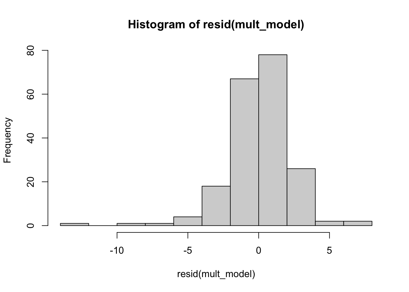
plot(fitted(mult_model), resid(mult_model))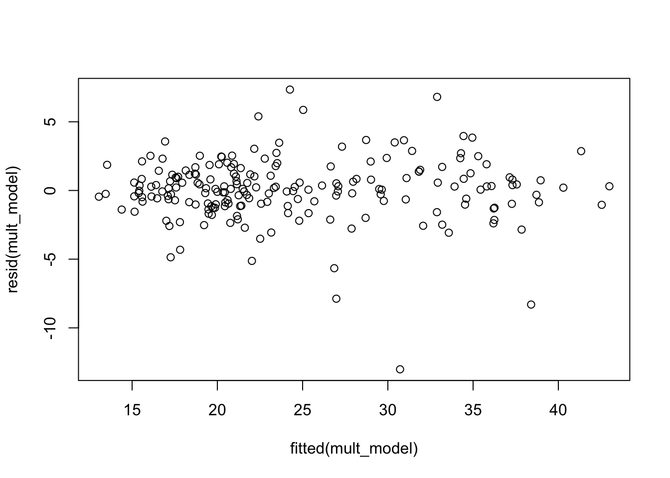
The histogram and residuals versus fitted both indicate that the residuals are more spread out (heavier tailed) than they should be if our model was 100 percent correct. The qq plot below is saying the same thing, since the plot is S shaped (with that orientation).
qqnorm(resid(mult_model))
qqline(resid(mult_model))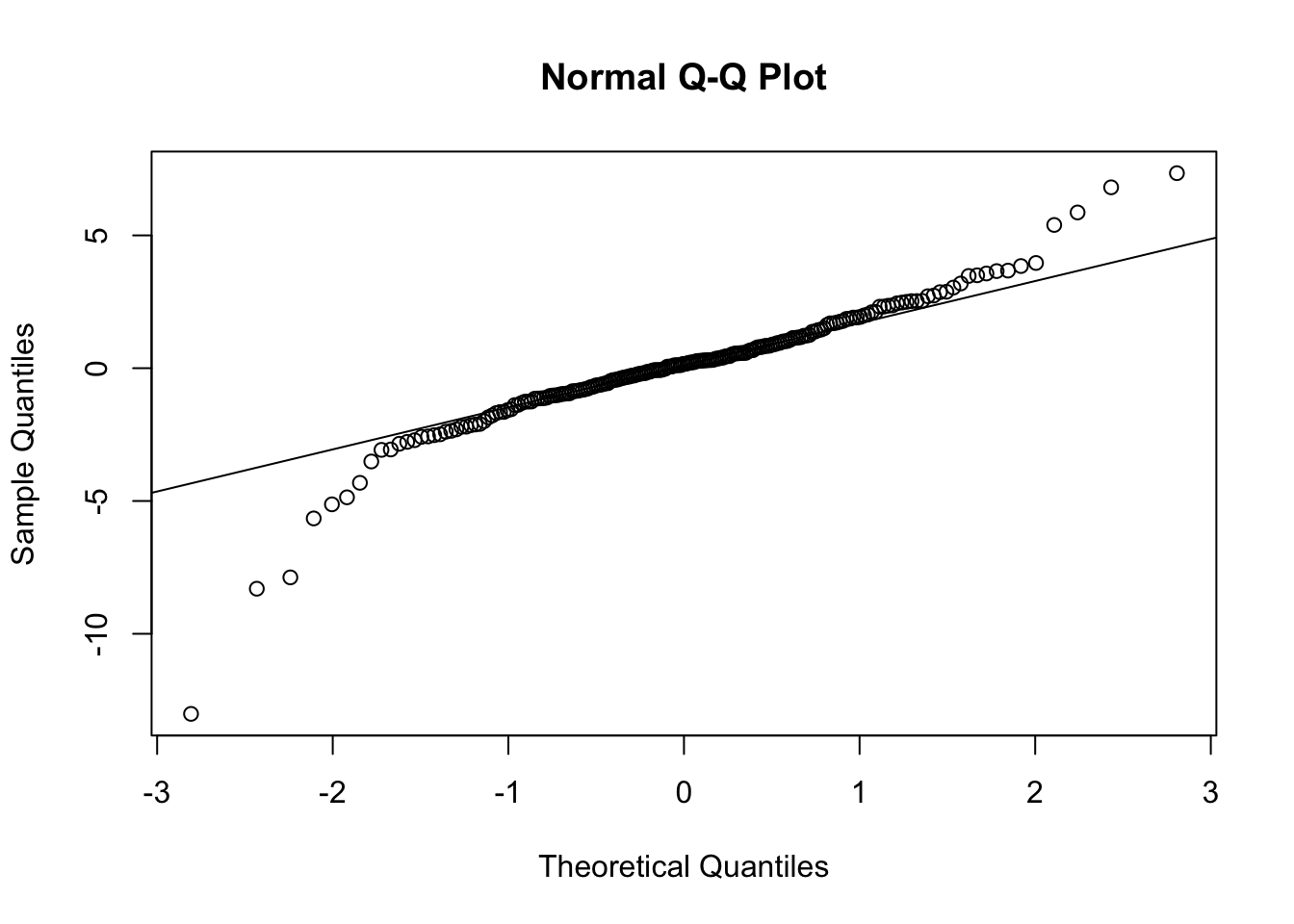
Looking at the residual plots like this is really checking our priors. Our model can be re-conceptualized as a linear model with student’s t error, and we assigned a prior probability of 0 to all degrees of freedom except \(\infty\), which corresponds to normal errors. Was that an informed decision? If so, then it really doesn’t matter (much) if the residuals don’t align with the priors.
In our case, however, it was not an informed decision. We simply wanted to use stan_glm with the default, which is normal errors. It makes sense to check after the fact whether that choice aligns well with the data.
Compare the model with all of the variables to the model with only location and temperature at 9 AM.
bayesrules::prediction_summary_cv(data = ww_mult, model = mult_model, k = 10)## $folds
## fold mae mae_scaled within_50 within_95
## 1 1 1.5396889 0.6520767 0.50 0.95
## 2 2 1.2664371 0.5589612 0.55 0.90
## 3 3 0.8193791 0.3521199 0.75 0.90
## 4 4 1.1871507 0.4930044 0.60 0.95
## 5 5 1.4352437 0.5940134 0.60 0.95
## 6 6 0.8359931 0.3449275 0.70 1.00
## 7 7 1.0273133 0.4658166 0.70 0.95
## 8 8 1.0977420 0.4454867 0.75 0.95
## 9 9 1.6161218 0.6634625 0.50 0.95
## 10 10 0.9626415 0.4045980 0.60 0.95
##
## $cv
## mae mae_scaled within_50 within_95
## 1 1.178771 0.4974467 0.625 0.945bayesrules::prediction_summary_cv(data = ww, model = model_9am, k = 10)## $folds
## fold mae mae_scaled within_50 within_95
## 1 1 1.0705824 0.4399713 0.65 0.95
## 2 2 1.2543266 0.5036930 0.70 1.00
## 3 3 0.8936940 0.3917622 0.80 0.95
## 4 4 1.1106273 0.4581024 0.70 1.00
## 5 5 1.1079987 0.4599255 0.70 0.90
## 6 6 1.6921752 0.7035072 0.50 0.95
## 7 7 0.9075976 0.3702463 0.55 1.00
## 8 8 1.1979440 0.4955176 0.70 0.95
## 9 9 0.7818788 0.3188865 0.70 0.90
## 10 10 0.8842594 0.3724907 0.60 0.95
##
## $cv
## mae mae_scaled within_50 within_95
## 1 1.090108 0.4514103 0.66 0.955We see that the mean absolute error in the out of bag predictions is smaller in the simpler model than in the more complicated model. The 50 percent prediction intervals are performing slighlty closer to their design in the full model than the simplified model, in that they true coverage is closer to the desired 50 percent coverage. Reasonable people can disagree on whether we prefer the model that has higher coverage or the model that has coverage closer to the designed coverage; I prefer coverage to match the designed prediction interval, so this measure would prefer the more complicated model.
Let’s see how to code up the MAE in the leave one out CV technique.
library(future.apply)
plan("multisession")
log_likes <- future_sapply(1:200, function(x) {
  small_dat <- ww_mult[-x, ]
  small_mod <- rstanarm::stan_glm(temp3pm ~ ., data = small_dat, refresh = 0)
  test_dat <- ww_mult[x, ]
  # tidybayes::spread_draws(small_mod, `[\\(a-z].*`, regex = T) %>%
  #   janitor::clean_names() %>%
  #   mutate(predict = intercept + location_wollongong * (test_dat$location == "Wollongong") + windspeed9am * test_dat$windspeed9am +
  #                            humidity9am * test_dat$humidity9am + pressure9am * test_dat$pressure9am + temp9am * test_dat$temp9am) %>%
  #   pull(predict) %>%
  #   mean()
  predict(small_mod, newdata = ww_mult[x, ])
}, future.seed = TRUE)
mean(abs(log_likes - ww_mult$temp3pm))
## [1] 1.594102log_likes_2 <- future_sapply(1:200, function(x) {
small_dat <- ww_mult[-x, ]
small_mod <- rstanarm::stan_glm(temp3pm ~ temp9am + location, data = small_dat, refresh = 0)
test_dat <- ww_mult[x, ]
# tidybayes::spread_draws(small_mod, `[\\(a-z].*`, regex = T) %>%
# janitor::clean_names() %>%
# mutate(predict = intercept + location_wollongong * (test_dat$location == "Wollongong") + temp9am * test_dat$temp9am) %>%
# pull(predict) %>%
# mean()
predict(small_mod, newdata = ww_mult[x, ])
}, future.seed = TRUE)
mean(abs(log_likes_2 - ww_mult$temp3pm))## [1] 1.593015plan("sequential")Compare the model with all of the variables to the model with only location and temperature at 9 AM.
This is the same example as above, but we are using a different technique. Here, we use the loo function from rstanarm to estimate the leave-one-out cross validation errors.
loo_all <- rstanarm::loo(mult_model)
loo_some <- rstanarm::loo(model_9am)
We only look at some of the information output from this. First, elpd_loo is the expected log predictive densities of the out of bag samples.5 Recall when we were counting the percentage of out of bag samples in the 50 percent posterior predictive intervals, we said it might be better to compute the posterior likelihoods of all possible new data and use that information. Well, that is what we are doing now, but we don’t provide details.
loo::loo_compare(loo_all, loo_some)## elpd_diff se_diff
## mult_model 0.0 0.0
## model_9am -3.6 4.1The higher the value of the expected log predictive density, the better. In this case, we see that the model only using location and temperature at 9 AM is 3.4 units worse than the model using all of the data. The rule of thumb suggested is that in order for a more complicated model to be chosen, its ELPD needs to be 2 standard errors larger than the simpler model. In this case, the difference is 3.4, and the standard error is 4.0, so we would choose the simpler model even though it has a worse ELPD.
This is all we will be using the ELPD for; comparing two models in this fashion.
4.3 Bias-variance tradeoff
Due to popular demand, I am adding this brief section to illustrate why it is sometimes better to ignore some predictor variables in order to minimize the error in predicted values. The basic idea is the bias-variance tradeoff. In this form, it says that the mean squared error of future predictions can be broken down into three components, the inherent variance of the data (which cannot be accounted for), the bias of the model squared, and the variance of the model. One strategy is to find the unbiased model which has the smallest variance. One might think that this would lead to the model with the lowest mean squared error, but many times we can increase the bias while decreasing the model variance by a larger amount. Here is a simple example that illustrates the idea.
Suppose your data is generated by \(y = 1 + \epsilon\), where \(\epsilon \sim N(0, \sigma = 10)\). We have two competing models:
- the first model is just that we always predict zero.
- the second model is that we draw a step function through all of the \((x, y)\) pairs and that gives us our prediction.
We note that the first model is biased in the sense that the expected value of the prediction (which is 0) is not the same as the expected value of the response (which is 1). However, it has very low variance. The variance of the model is 0; we always use the same model no matter what data we get. According to our formula, the mean squared error should be 100 + 1 = 101. We can run the following code a few times to check that the mean squared error is approximately 101.
y <- rnorm(100000, 1, 10)
mean((y - 0)^2)
## [1] 100.528In the second model, the bias is 0, the expected value of the prediction is 1. However, the variance of the prediction is the same as the variance of the data, which in this case is 100, so our total MSE would be 200.
x <- runif(20, 0, 1)
y <- 1 + rnorm(20, 1, 10)
f <- approxfun(x, y, method = "constant", yright = y[which.max(x)], yleft = y[which.min(x)])
plot(x, y, xlim = c(0, 1))
curve(f, add = T, n = 5000)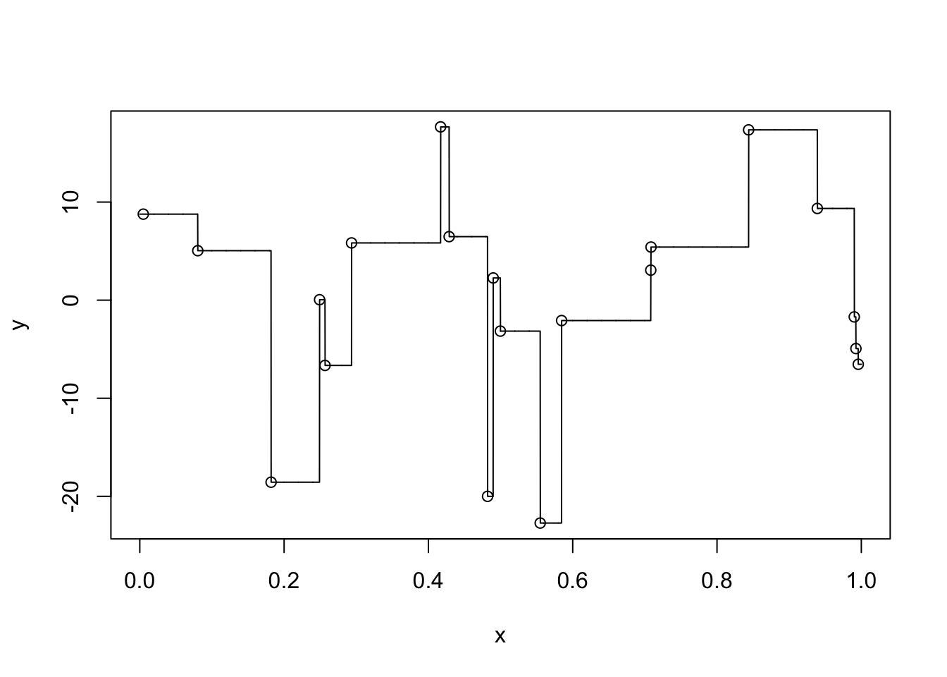
Let’s do this again with different data following the same generative process and see that we get quite a different model. That is what we mean by the variance of the model.
curve(f(x), col = 2, lty = 2, ylim = c(-25, 25))
x <- runif(20, 0, 1)
y <- 1 + rnorm(20, 1, 10)
f <- approxfun(x, y, method = "constant", yright = y[which.max(x)], yleft = y[which.min(x)])
curve(f, add = T, col = 3, lty = 3)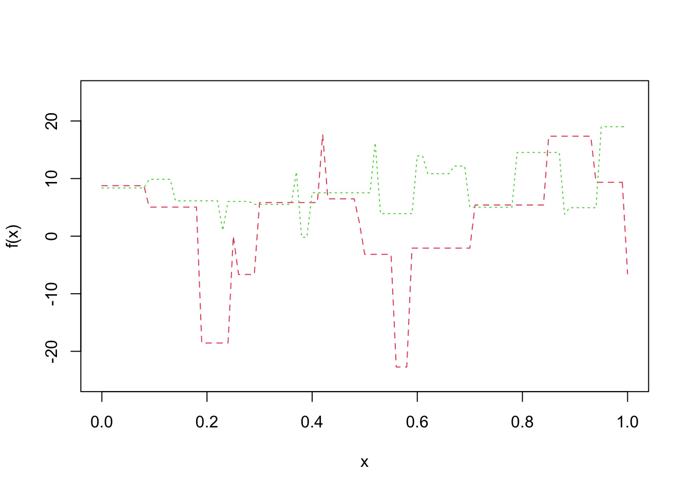
Let’s check the MSE with a simulation:
mean(replicate(10000, {
  x <- runif(20, 0, 1)
  y <- 1 + rnorm(20, 1, 10)
  f <- approxfun(x, y, method = "constant", yright = y[which.max(x)], yleft = y[which.min(x)])
  new_data <- 1 + rnorm(1, 1, 10)
  prediction <- f(runif(1, 0, 1))
  (new_data - prediction)^2
}))
## [1] 201.1697If you do this several times, you will see that the MSE is about 200.
How does this relate to variable selection? If you have a predictor that is “weakly predictive” in the sense that the prediction will be biased if you don’t include the predictor, but the variance in the coefficient associated with the predictor is large relative to the amount of bias it removes, then removing that predictor from the model will cause the MSE to decrease.
4.4 Exercises
Consider the retinal thickness data, which you can download [here](You can download the data set here. Recall that we cleaned up the data as follows, after reading in with read.csv.
dd <- dd %>%
  mutate(across(.fns = function(x) str_replace(x, ",", "."))) %>%
  mutate(across(.fns = function(x) as.numeric(x))) %>%
  janitor::clean_names()

dd <- dd %>%
  mutate(onl_mean = (onl_inner + onl_outer) / 2)
Change
sexto be a factor. Can you determine what the values 0 and 1 mean? Can you think of a better way to have coded this data?Plot
onl_meanversusage, with color determined bysex, and a line of best fit through each group.Create a linear model of
onl_meanonageandsex, with no interaction.If \(\mathrm{onl\_mean} = \beta_0 + \beta_1 \times \mathrm{age} + \beta_2 \times \mathrm{sex} + \epsilon\), where \(\epsilon \sim N(0, \sigma)\), provide mean values for \(\beta_0, \beta_1, \beta_2\), and \(\sigma\) from the posterior draws.
Use
spread_drawsto find a 90 percent posterior predictive interval foronl_meanfor a person withsex = 1andage = 30.Use
bayesrules::prediction_summary_cvto estimate the coverage of a 90 percent posterior prediction interval.Use
rstanarm::loo_compareto compare the model with age and sex to the model with just age, and to make a recommendation as to which model to choose.
This exercise is for graduate students only.
If you are doing the data analysis, then find a variable that makes sense as a response, and a metric and a categorical predictor. Explore modeling the response only on the metric predictor, on both the metric and the categorical predictor, and on both predictors together with their interaction. Provide illustrative plots and explain which of the three models you would recommend.
If you are doing the coding, write code that implements 10-fold cross validation to estimate the coverage of a 50 percent posterior predictive interval. Split the data set into 10 random, evenly sized pieces. Take turns removing one of the pieces and building the model on the other 9 pieces combined. Estimate the coverage on the pieces that have been removed. Apply your code to the retinal thickness data to estimate the coverage of a 50 percent ppi when
onl_meanis described byage.Theory Jeffreys’ prior. When we have a random variable \(X\) that depends on a single parameter \(\theta\) in a model, Jeffrey proposed the following noninformative prior for \(\theta\): \[ J(\theta) = \sqrt{-E\left[\frac{d^2 \log f(X|\theta)} {d\theta^2} \right]} \] where \(f\) is the probability density or mass function. Find Jeffreys’ prior for the parameter \(\pi\), the probability of success in a binomial random variable with \(n\) trials.
out of bag samples are the ones that are left out when doing leave one out cross validation, or more generally, any kind of cross validation.↩︎