Chapter 7 Hierarchical Models
In this chapter, we introduce hierarchical models through first doing a hierarchical model for probability of success, and then a motivating example for a more general case.
7.1 Probability of Success
In this section, we return to the coin flipping example from earlier. Thirteen medical students were given instructions to “try to toss heads” and given a few minutes to practice. They then tossed a coin 300 times and the number of heads was observed.
This section should be considered an exploration of ideas. The final product presented still has issues.
bayeta::coins## id heads tails
## 1 1 162 138
## 2 2 175 125
## 3 3 159 141
## 4 4 179 121
## 5 5 203 97
## 6 6 168 132
## 7 7 170 130
## 8 8 160 140
## 9 9 192 108
## 10 10 167 133
## 11 11 154 146
## 12 12 153 147
## 13 13 176 124In this experiment, we aren’t necessarily interested just in these thirteen people and how their probability of tossing heads. Let \(\theta_1, \ldost, \theta_{13}\) be the 13 probabilities of getting heads from the participants. We might imagine that there is a parent distribution \(p(\varphi)\) that these 13 probabilities are drawn from. Since we will be doing these computations by hand, we only consider the first 3 participants.
We observe 162, 175 and 159 heads out of 300 tosses in the first three participants. As usual, we are interested in the probability of the parameters given the data, but in this case, we need to say what the parameters in question are. As a refresher, lets remind ourseleves what we would have done with only one participant. Let \(\theta\) be the probability of getting heads, and we put a beta(1,1) prior on \(\theta\).
\[\begin{align*} f(\theta|162 H) \propto f(162 H|\theta) f(\theta) = \mathrm{dbinom(162, 300, theta) dbeta(theta, 1, 1)} \end{align*}\]
Now, with 3 values
\[\begin{align*} f(\theta_1, \theta_2, \theta_3, \alpha, \beta|162 H, 175 H, 159 H) &\propto f(162 H, 175 H, 159 H|\theta_i, \alpha, \beta) f(\theta_i, \alpha, \beta) \\ &= f(162 H, 175 H, 159 H|\theta_i) f(\theta_i| \alpha, \beta) f(\alpha, \beta) \\ &= \mathrm{dbinom(162, 300, theta1) * dbinom(175, 300, theta2) * dbinom(159, 300, theta3) * dbeta(theta1, alpha, beta) * dbeta(theta2, alpha, beta) * dbeta(theta3, alpha, beta)} f(\alpha, \beta) \end{align*}\]
Here, we are requiring that the probability function of the data only depends on \(\theta_i\), not on how those \(\theta_i\) came to be from the parent distribution. We can also see that we need to specify \(f(\alpha, \beta)\), which we will assume is equal to \((\alpha) f(\beta)\). Sometimes we will wish to have a vague prior on \(\alpha\) and \(\beta\), but notice that \(\alpha\) and \(\beta\) can take on any real value, so we can’t make it uniform. There are several possibilities here.
This does not work well.
One that is mentioned in this book as *problematic is to let \(\alpha\) and \(\beta\) be uniformly distributed on a region. We could make a transformation of \(\mathrm{logit}\left(\frac{\alpha}{\alpha + \beta}\right)\) (the logistic function of the mean) and \(\log(\alpha + \beta)\) (the log of the “sample size”). We might reasonably guess that the mean would be between 0.3 and 0.7, which leads to the logistic function of the mean being between \(-0.8\) and \(0.8\), while the sample size is harder to estimate, but perhaps we can say it is between 5 and 20 to start, so the log of the sample size is between 1.5 and 3. For \(\theta_1, \ldots, \theta_3\) we take a grid between 0.5 and 0.7. This gives us a five-dimensional** grid to sample from, so we won’t expect our results to be spectacular.
After looking at the data and playing with this more, we can do better with the sample size. Surely the min and max of 3 samples are unlikely to be more than 6 standard deviations apart. Looking at the standard deviation of a beta random variable, this says \(0.1^2 \approx \frac{.25}{s^3}\), where \(s = \alpha + \beta\). Solving for \(\alpha + \beta\) yields that \(\alpha + \beta \le 10\). So log of that is about 3.
grid <- expand.grid(seq(-0.2, 0.5, length.out = 16), seq(1, 3, length.out = 16), seq(.45, .65, length.out = 20), seq(.45, .7, length.out = 19), seq(.43, .63, length.out = 21))

post <- function(logisticmean, logsize, theta1, theta2, theta3) {
  beta <- exp(logsize) / (1 + exp(logisticmean))
  alpha <- beta * exp(logisticmean)
  prod(dbinom(c(162, 175, 159), 300, c(theta1, theta2, theta3))) * prod(dbeta(c(theta1, theta2, theta3), alpha, beta))
}

grid$prob <- sapply(1:nrow(grid), function(x) {
  post(grid$Var1[x], grid$Var2[x], grid$Var3[x], grid$Var4[x], grid$Var5[x])
})

samples <- sample(1:nrow(grid), 10000, T, prob = grid$prob)
ggplot(grid[samples, ], aes(Var1, Var2)) +
  geom_jitter()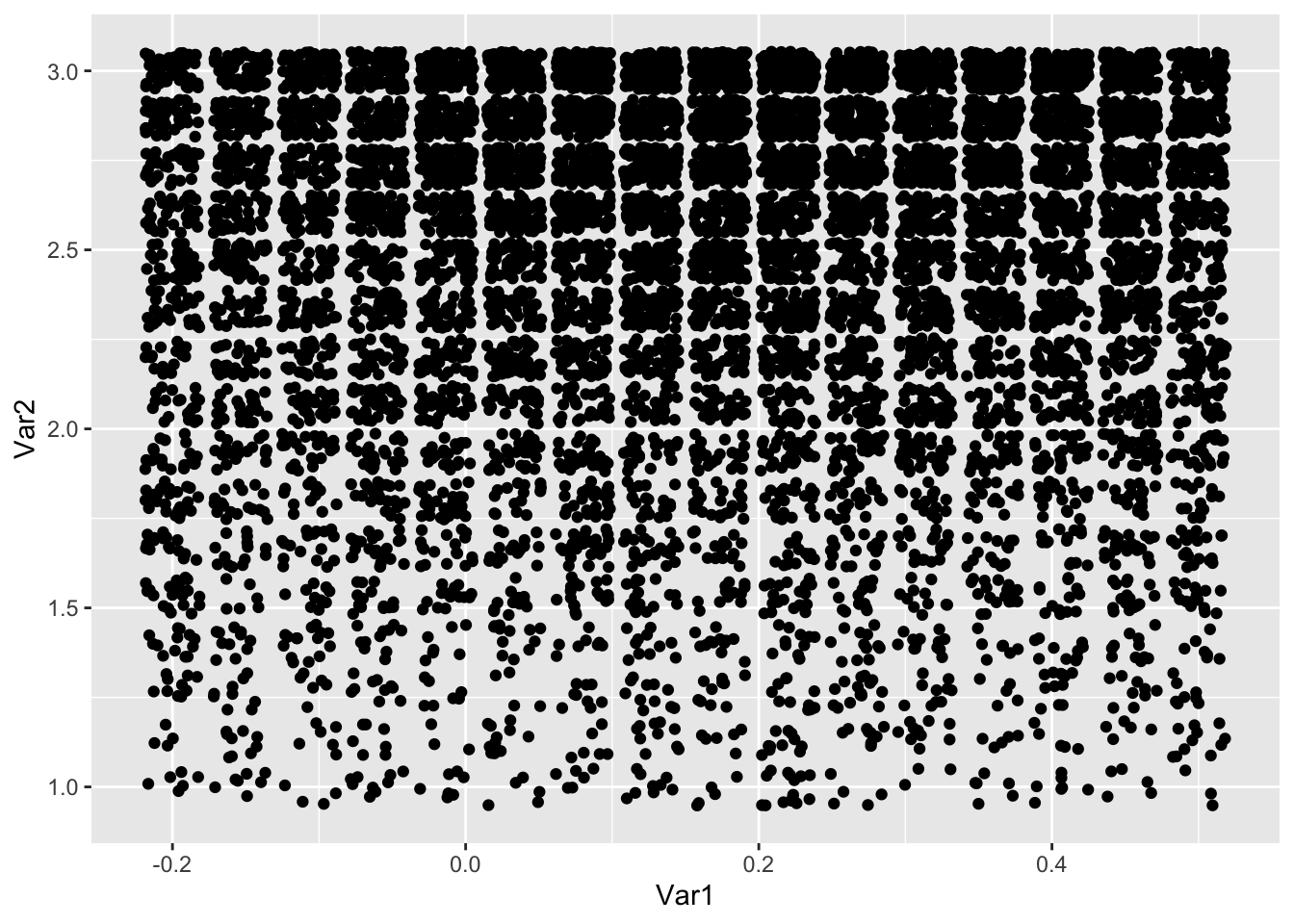
plot(grid[samples, c("Var1", "Var2")])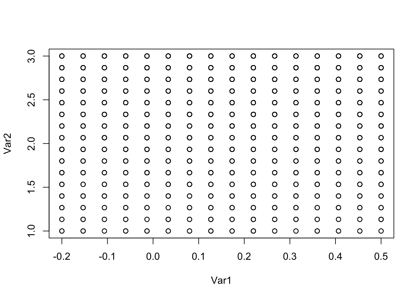
hist(grid[samples, "Var1"])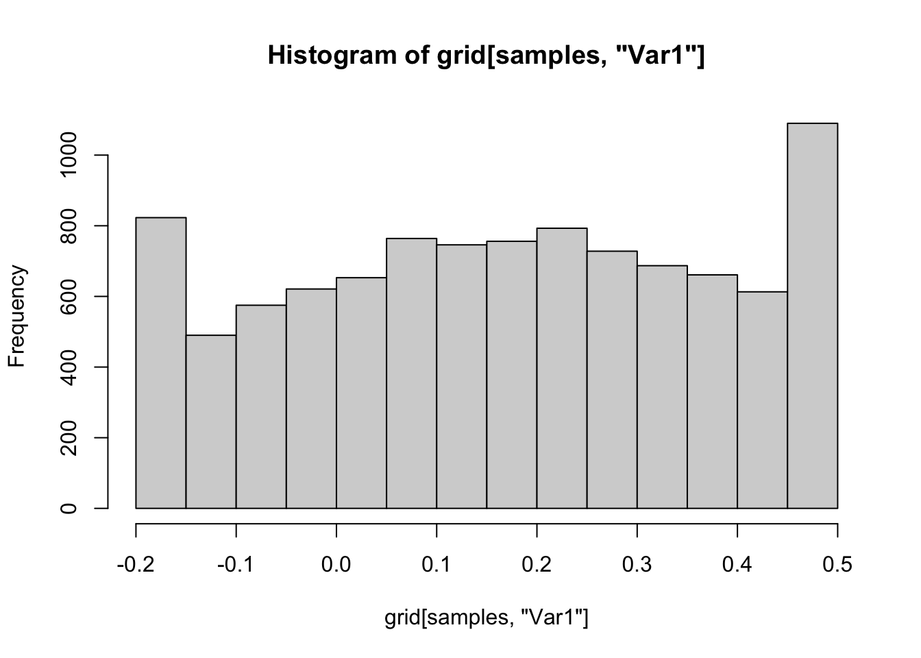
hist(grid[samples, "Var2"])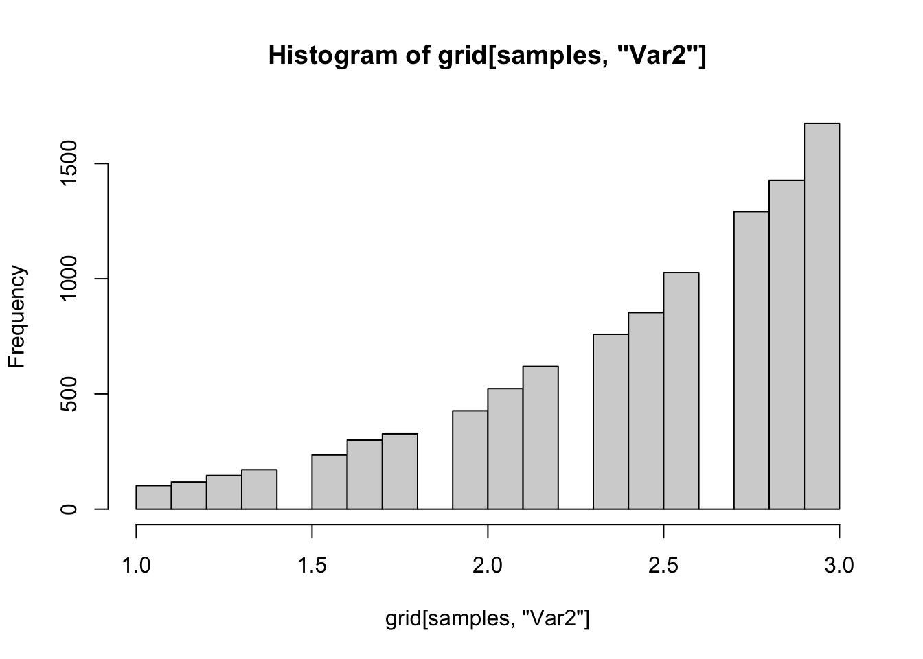
hist(grid[samples, "Var3"])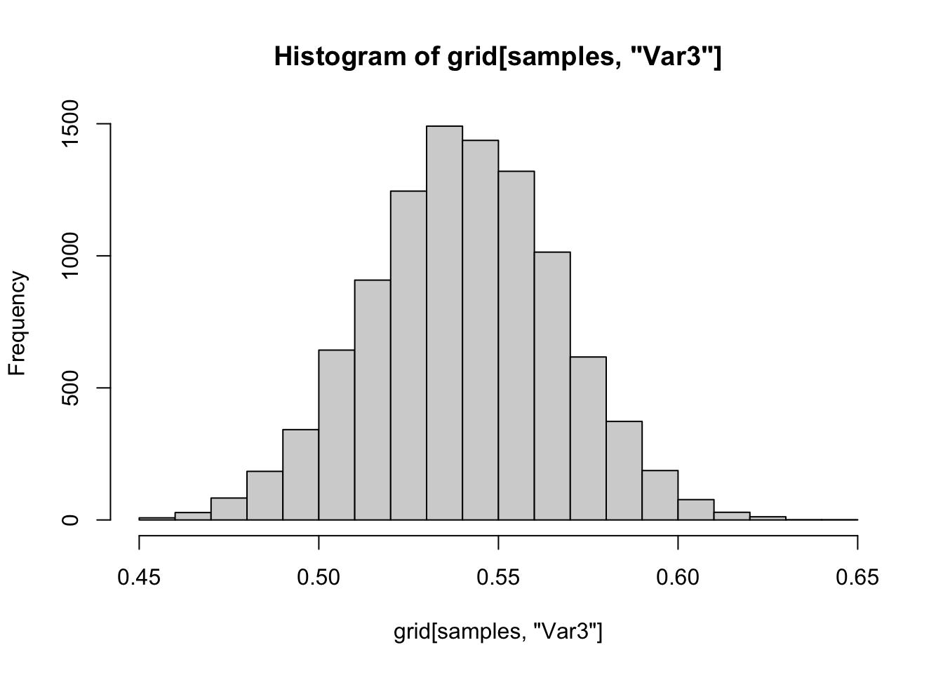
hist(grid[samples, "Var4"])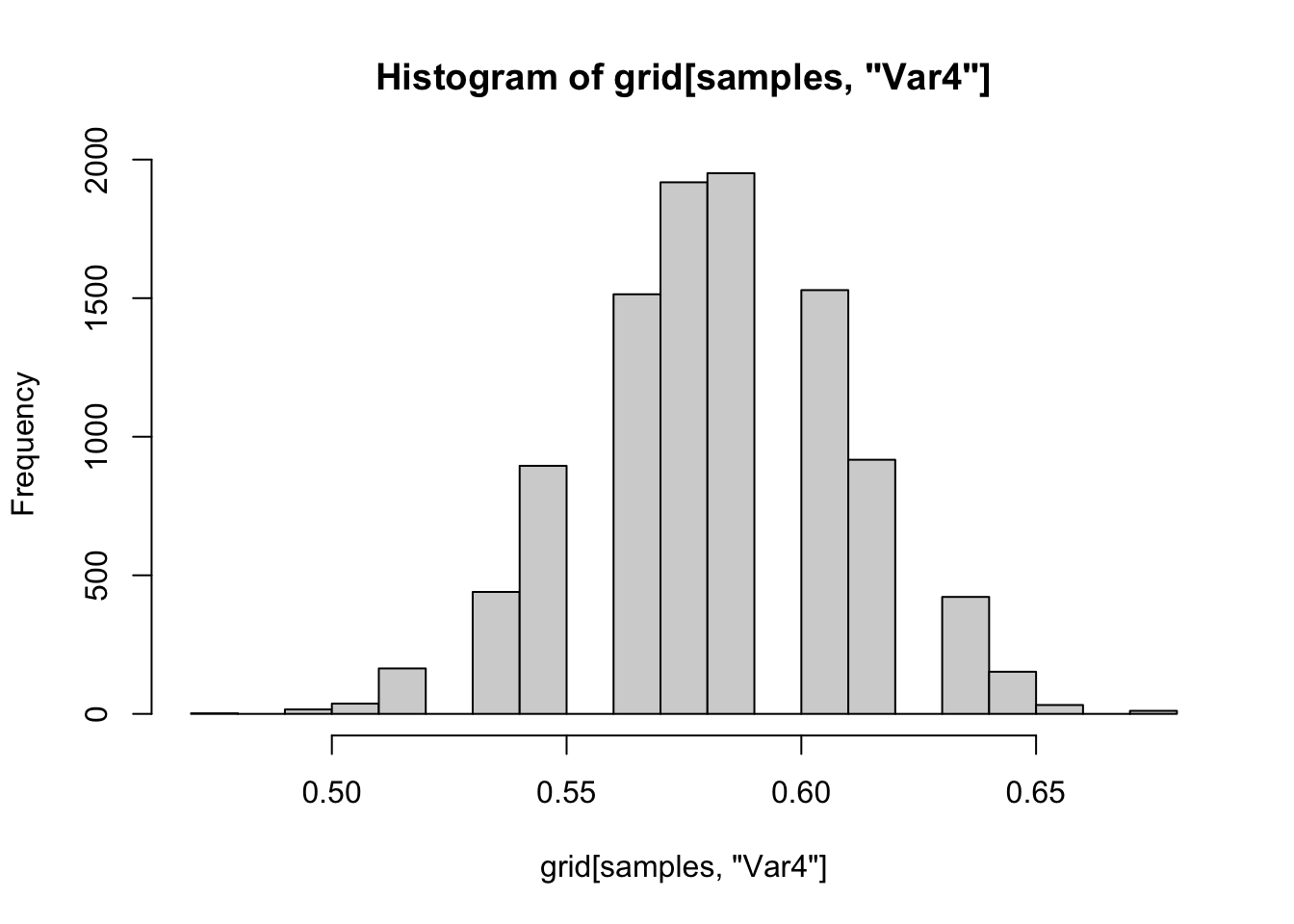
hist(grid[samples, "Var5"])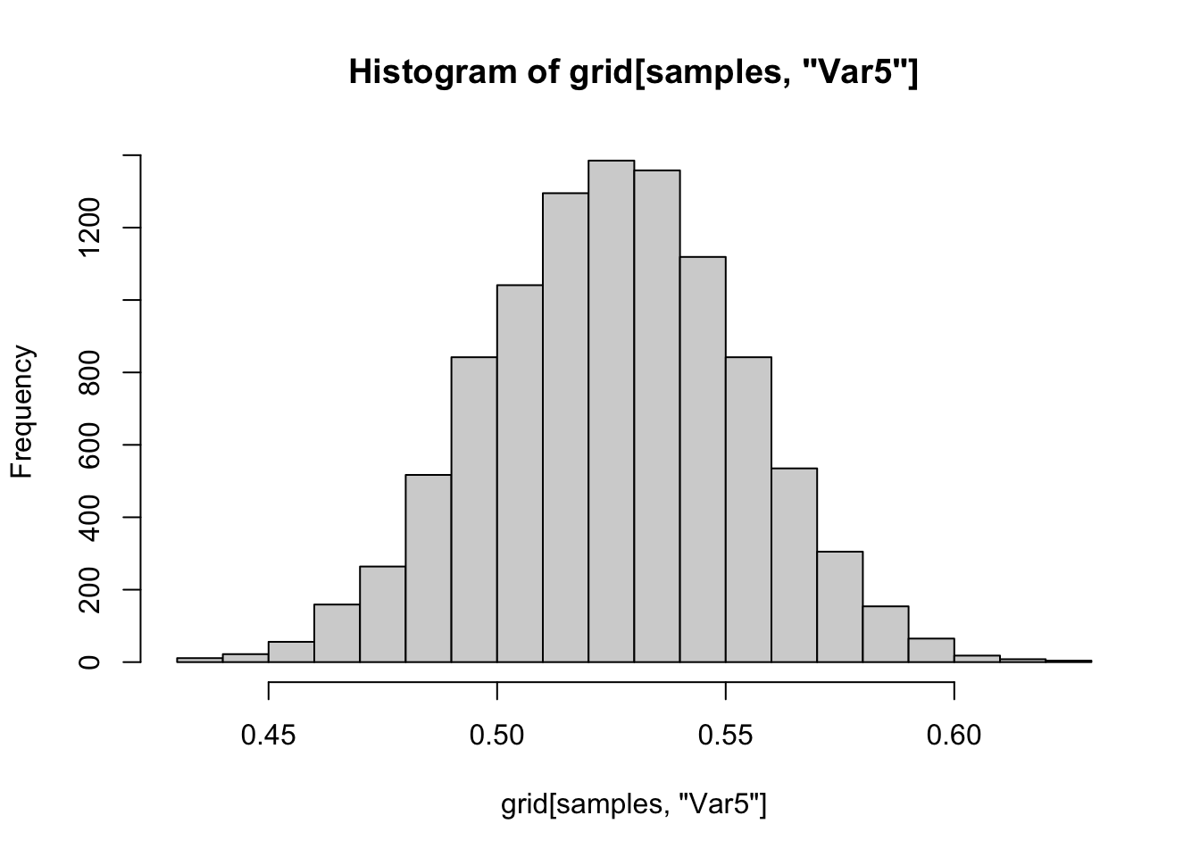
logisticmean <- grid[samples, "Var1"]
logsize <- grid[samples, "Var2"]

beta <- exp(logsize) / (1 + exp(logisticmean))
alpha <- beta * exp(logisticmean)

HDInterval::hdi(beta)
## lower upper
## 1.347149 9.875404
## attr(,"credMass")
## [1] 0.95HDInterval::hdi(alpha)## lower upper
## 1.570348 11.603388
## attr(,"credMass")
## [1] 0.95HDInterval::hdi(alpha / (alpha + beta))## lower upper
## 0.4617416 0.6224593
## attr(,"credMass")
## [1] 0.95HDInterval::hdi(grid[samples, "Var3"])## lower upper
## 0.4921053 0.5973684
## attr(,"credMass")
## [1] 0.95HDInterval::hdi(grid[samples, "Var4"])## lower upper
## 0.5333333 0.6305556
## attr(,"credMass")
## [1] 0.95HDInterval::hdi(grid[samples, "Var5"])## lower upper
## 0.48 0.58
## attr(,"credMass")
## [1] 0.95Note that when we plot the draws, we get the majority of our draws are close to the sample size 3 threshold. Many times, we would increase the sample size here because it looks like our prior isn’t weakly informative. However, we need to decide whether we really think we happened to get 3 draws that have the max and min more than 6 standard deviations apart, or whether something else is going on. For the sake of argument, let’s imagine we allowed sample size to get as large as we want. Note that for fixed values of \(\theta_i\), prod(dbinom(c(162, 175, 159), 300, c(theta1, theta2, theta3))) is a constant. So, if we pick \(\alpha\) and \(\beta\) so that \(\theta_i\) are all equal to the mode of beta with parameters \(\alpha\) and \(\beta\), then prod(dbeta(c(theta1, theta2, theta3), alpha, beta)) goes to \(\infty\). This is not what we want. In the code below, we let alpha and beta go to infinity and see that the posterior also goes to infinity. This says if we let \(\alpha + \beta\) be as large as \(\log(2000000) \approx 14.5\), then we will be choosing values for our draw based on the large values of dbeta.
theta1 <- .5
theta2 <- .5
theta3 <- .5

alpha_beta <- c(100, 1000, 10000, 100000, 1000000)
sapply(alpha_beta, function(x) {
  post(log(x / x), log(x + x), theta1, theta2, theta3)
})
## [1] 4.819524e-04 1.529220e-02 4.837450e-01 1.529788e+01 4.837629e+02The solution suggested in the book is to use a weakly informative prior, which can make the posterior integrable, and remove the possibility that the \(\alpha\) and \(\beta\) will march off to infinity. We try, in the transformed scale \(p(\alpha, \beta) \propto \alpha \beta(\alpha + \beta)^{-5/2}\), but that might only work if we have a reasonably large amount of data. In which case, the grid method won’t work.
theta_length <- 12
other_length <- 16
grid <- expand.grid(
  seq(-0.2, 0.5, length.out = 16),
  seq(1, 12, length.out = 16),
  seq(.45, .63, length.out = theta_length),
  seq(.45, .63, length.out = theta_length),
  seq(.45, .63, length.out = theta_length),
  seq(.45, .63, length.out = theta_length)
)

post <- function(logisticmean, logsize, theta1, theta2, theta3, theta4) {
  beta <- exp(logsize) / (1 + exp(logisticmean))
  alpha <- beta * exp(logisticmean)
  prod(dbinom(c(162, 175, 159, 179), 300, c(theta1, theta2, theta3, theta4))) * prod(dbeta(c(theta1, theta2, theta3, theta4), alpha, beta)) * alpha * beta * (alpha + beta)^(-2.5)
}

vecpost <- Vectorize(FUN = post, vectorize.args = c("logisticmean", "logsize", "theta1", "theta2", "theta3", "theta4"))

grid$prob <- vecpost(grid$Var1, grid$Var2, grid$Var3, grid$Var4, grid$Var5, grid$Var6)

samples <- sample(1:nrow(grid), 10000, T, prob = grid$prob)
ggplot(grid[samples, ], aes(Var1, Var2)) +
  geom_jitter()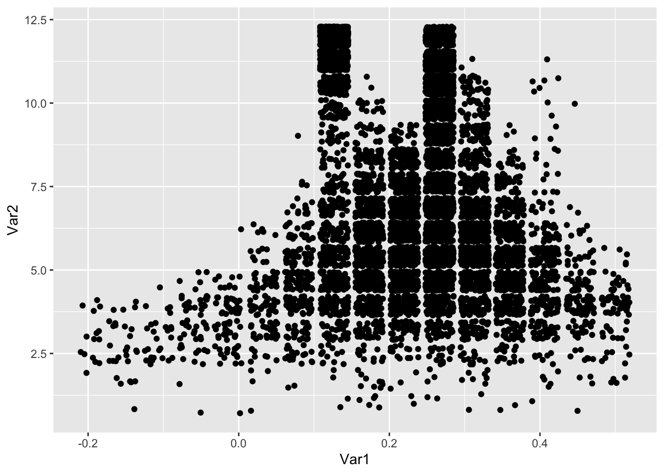
plot(grid[samples, c("Var1", "Var2")])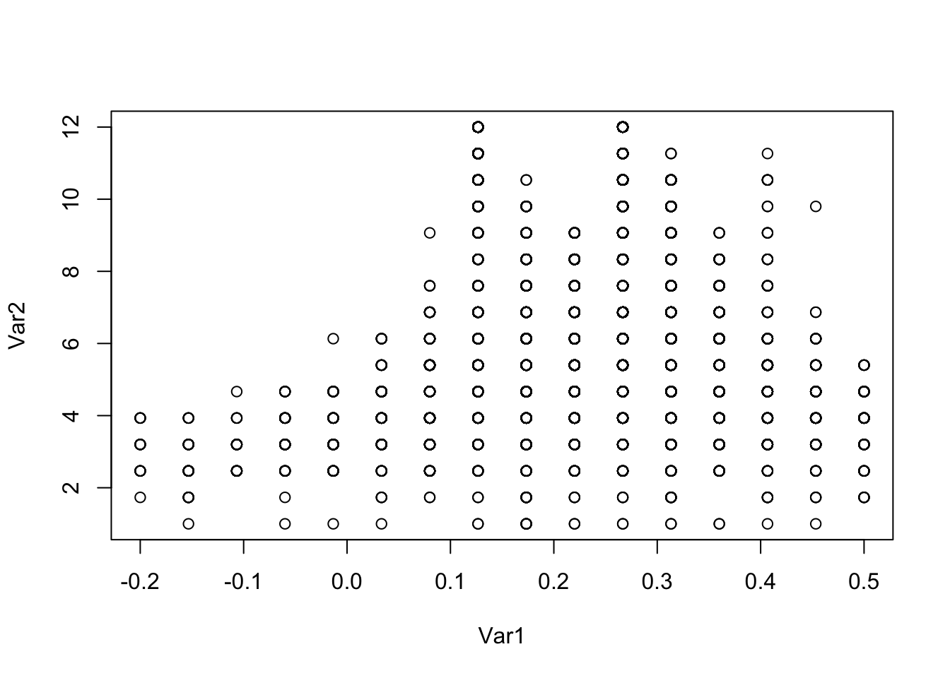
hist(grid[samples, "Var1"])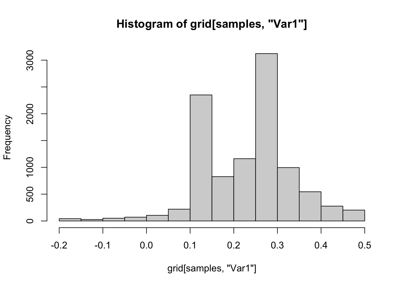
hist(grid[samples, "Var2"])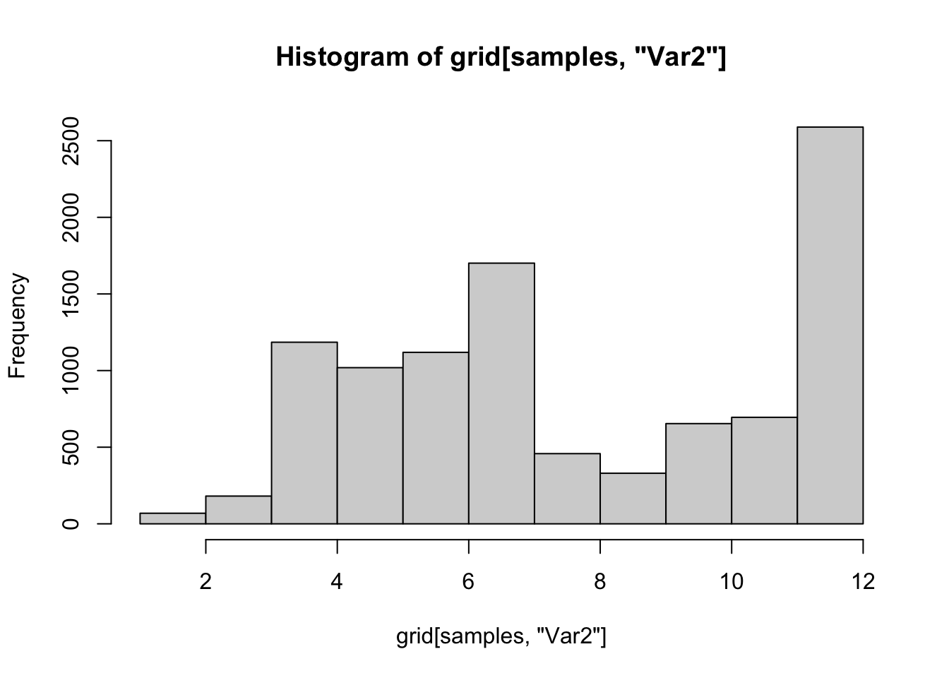
barplot(table(round(grid[samples, "Var3"], 3)))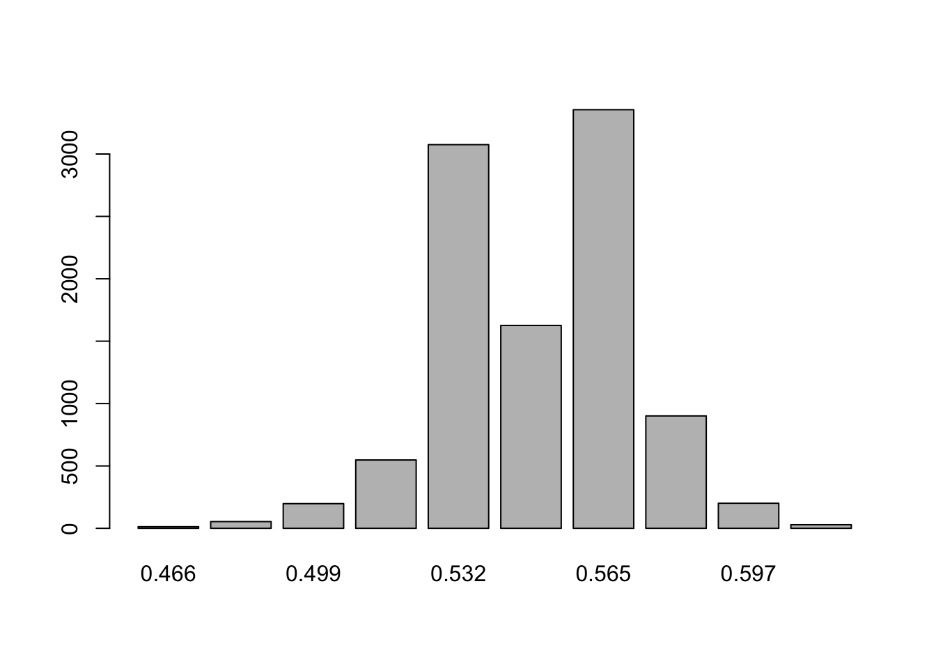
barplot(table(round(grid[samples, "Var4"], 3)))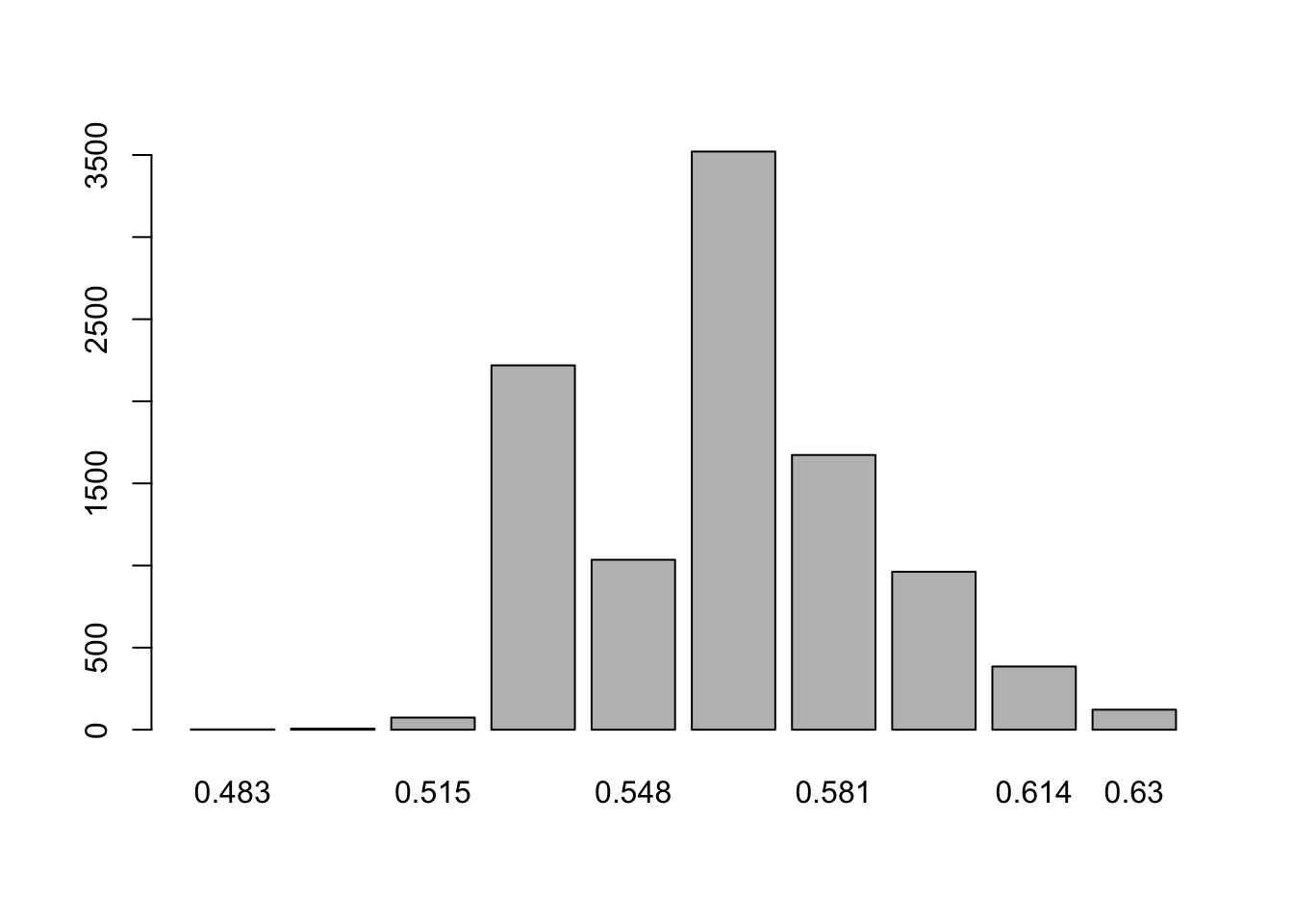
barplot(table(round(grid[samples, "Var5"], 3)))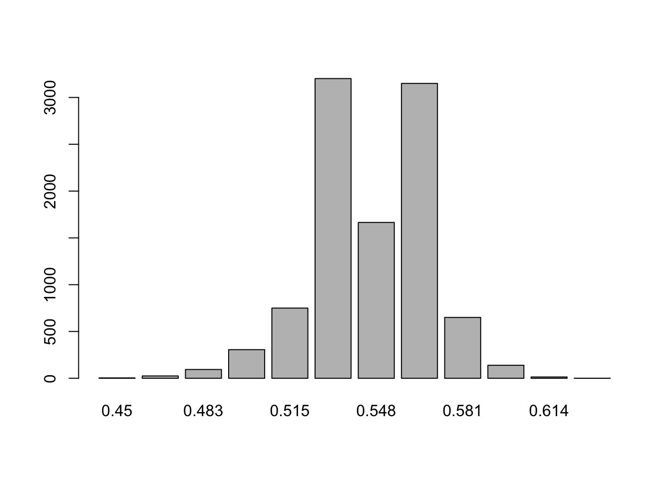
barplot(table(round(grid[samples, "Var6"], 3)))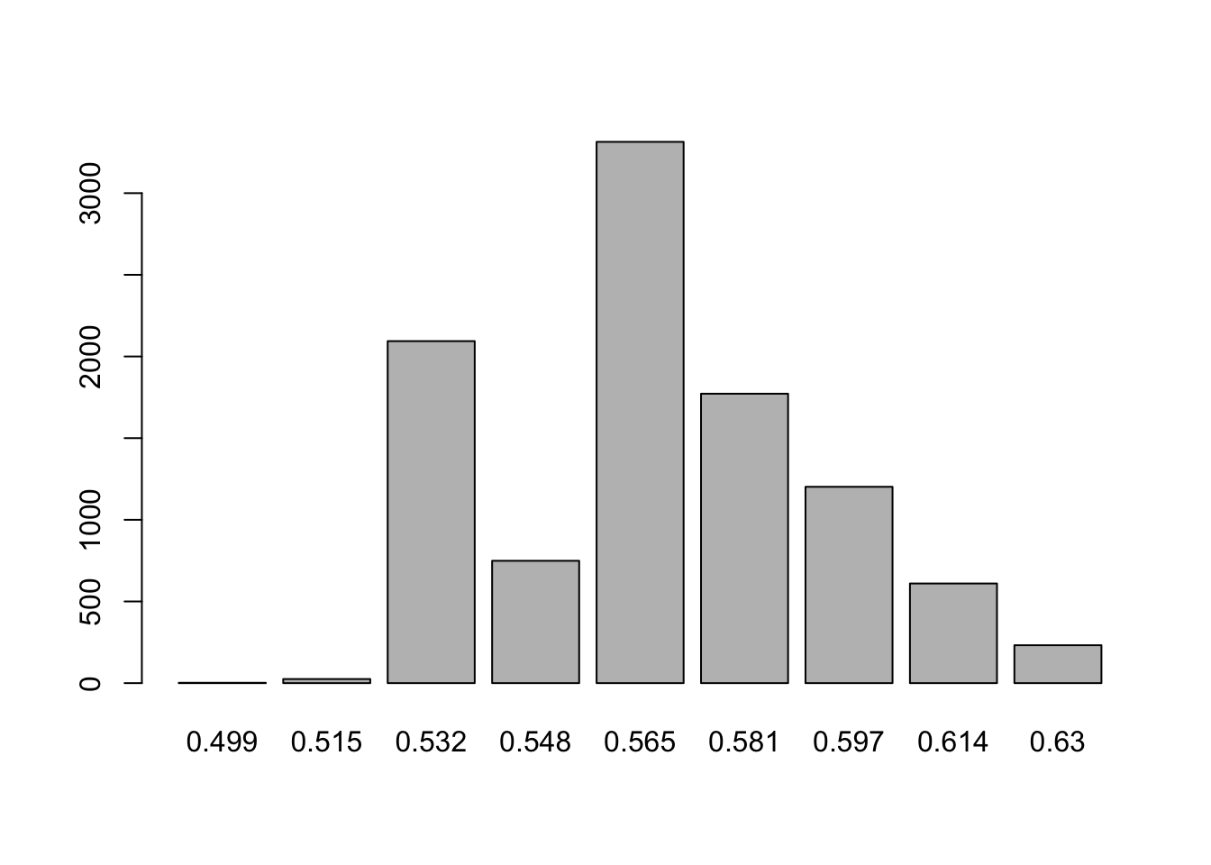
logisticmean <- grid[samples, "Var1"]
logsize <- grid[samples, "Var2"]

beta <- exp(logsize) / (1 + exp(logisticmean))
alpha <- beta * exp(logisticmean)

HDInterval::hdi(beta)
## lower upper
## 11.20584 76230.37390
## attr(,"credMass")
## [1] 0.95HDInterval::hdi(alpha)## lower upper
## 7.204561 86524.417519
## attr(,"credMass")
## [1] 0.95HDInterval::hdi(alpha / (alpha + beta))## lower upper
## 0.5199893 0.6114315
## attr(,"credMass")
## [1] 0.95HDInterval::hdi(alpha + beta)## lower upper
## 24.53253 162754.79142
## attr(,"credMass")
## [1] 0.95HDInterval::hdi(grid[samples, "Var3"])## lower upper
## 0.5154545 0.5809091
## attr(,"credMass")
## [1] 0.95HDInterval::hdi(grid[samples, "Var4"])## lower upper
## 0.5318182 0.6136364
## attr(,"credMass")
## [1] 0.95HDInterval::hdi(grid[samples, "Var5"])## lower upper
## 0.5154545 0.5972727
## attr(,"credMass")
## [1] 0.95Well, at least our draws don’t march off to infinity in this case, but \(\alpha + \beta\) still seems pretty large, and the posterior still goes to infinity if we take large enough values of \(\alpha + \beta\) and carefully chosen values of \(\theta_i\).
theta1 <- .5
theta2 <- .5
theta3 <- .5
theta4 <- .5

alpha_beta <- c(100, 1000, 10000, 100000, 1000000, 10^30)
sapply(alpha_beta, function(x) {
  post(log(x / x), log(x + x), theta1, theta2, theta3, theta4)
})
## [1] 1.596863e-08 5.072498e-07 1.604787e-05 5.075010e-04 1.604866e-02
## [6] 1.604867e+347.2 Linear regression with normal error
We consider the cherry_blossom_sample data set in the bayesrules package. Let’s examine it.
runners <- bayesrules::cherry_blossom_sampleWe are interested in determining the effect of age on running times for runners in their 50s and 60s, such as this group.
ggplot(runners, aes(age, net)) +
  geom_point() +
  geom_smooth(method = "lm", se = FALSE)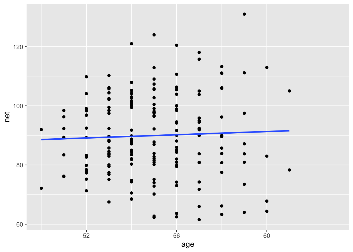
There are several ways that we could model this. Following the text, we split it into three different groups:
- Complete pooling. In this model, we lump all of the data together.
- No pooling. In this model, we consider each participant completely separately.
- Partial pooling. In this model, we imagine that there is a parent distribution that determines the proportion of heads that people will obtain when trying to get heads with the training provided in this experiment. Some people will be better at it than others, but there is some distribution to these probabilities.
Complete pooling. In this scenario, we pool all of the participants together into one big group. We ignore any possibility that people may differ in how age affects the time to complete the race.
library(rstanarm)
pooled_model <- stan_glm(net ~ age,
  data = runners,
  family = gaussian,
  prior = normal(0, 2.5, autoscale = TRUE),
  prior_intercept = normal(0, 2.5, autoscale = TRUE),
  prior_aux = exponential(1, autoscale = T),
  refresh = 0
)

bayesplot::mcmc_acf(pooled_model)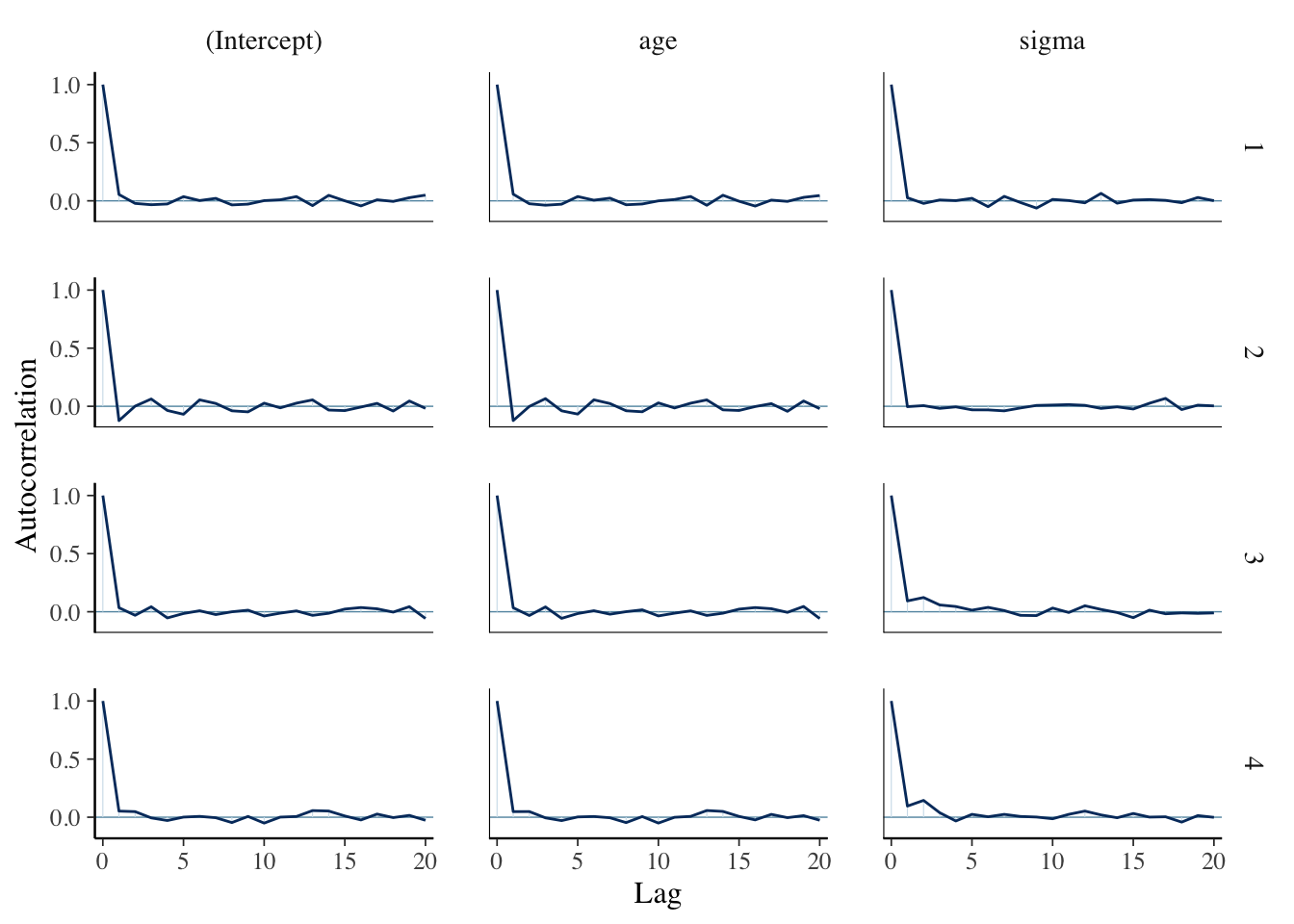
bayesplot::mcmc_trace(pooled_model)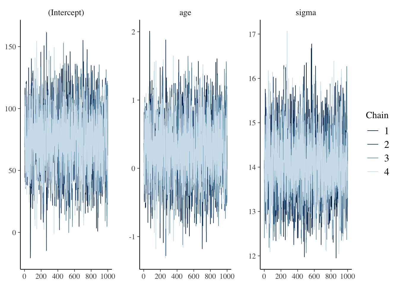
bayesplot::mcmc_dens_chains(pooled_model)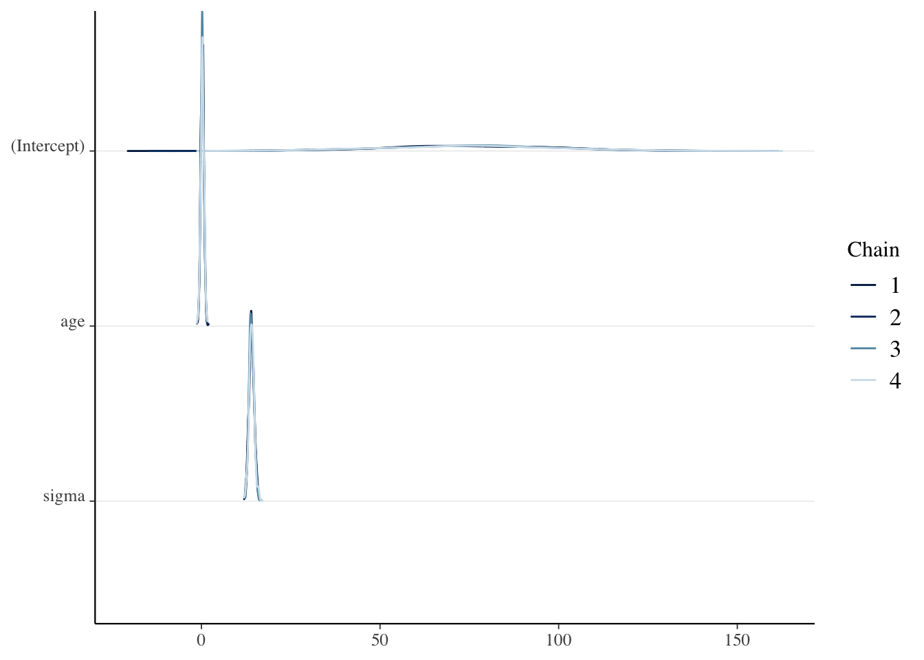
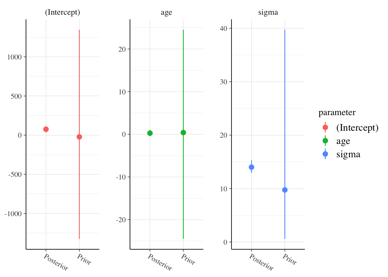
posterior_vs_prior(pooled_model,
  facet_args = list(scales = "free"),
  group_by_parameter = T
)
pp_check(pooled_model)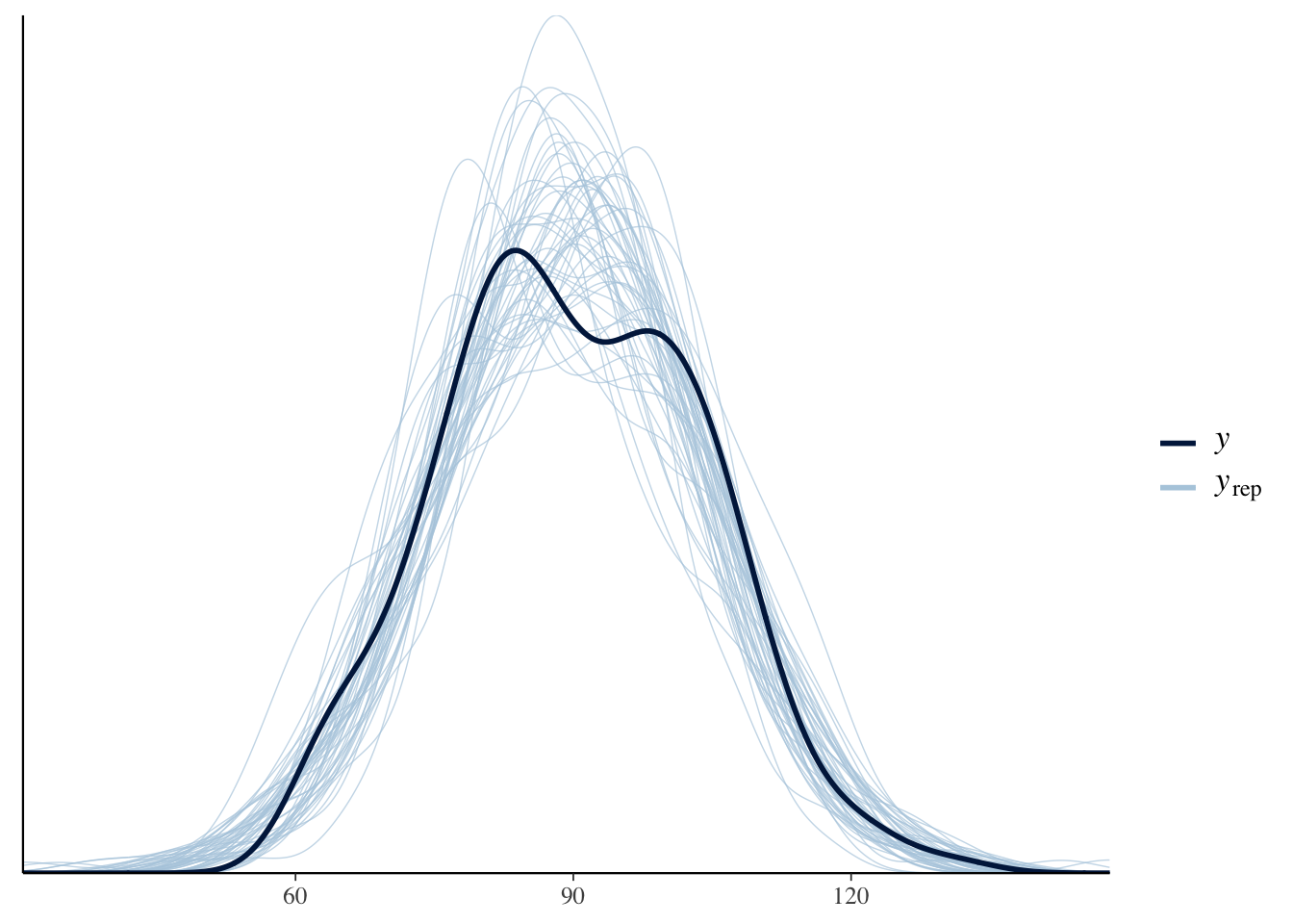
Let’s see whether the age variable is a significant predictor of the net time to run the race.
broom.mixed::tidy(pooled_model, conf.int = T, conf.level = 0.9)## # A tibble: 2 × 5
## term estimate std.error conf.low conf.high
## <chr> <dbl> <dbl> <dbl> <dbl>
## 1 (Intercept) 75.2 24.8 33.7 115.
## 2 age 0.265 0.443 -0.458 1.03No, it is not. This is perhaps surprising, because it goes against what common sense would say. But, it is also possible that the noise that is the individual variation of runners is overwhelming the relatively weak signal that is the age effect.
No pooling. In this model, we assume the effect of age on net time to run the race is independent for each person. The only parameter that is shared between the runners is sigma, which we assume is the same for all runners.
ggplot(runners, aes(age, net, group = runner)) +
  geom_point() +
  geom_smooth(method = "lm", se = F, color = "lightblue") +
  theme_minimal()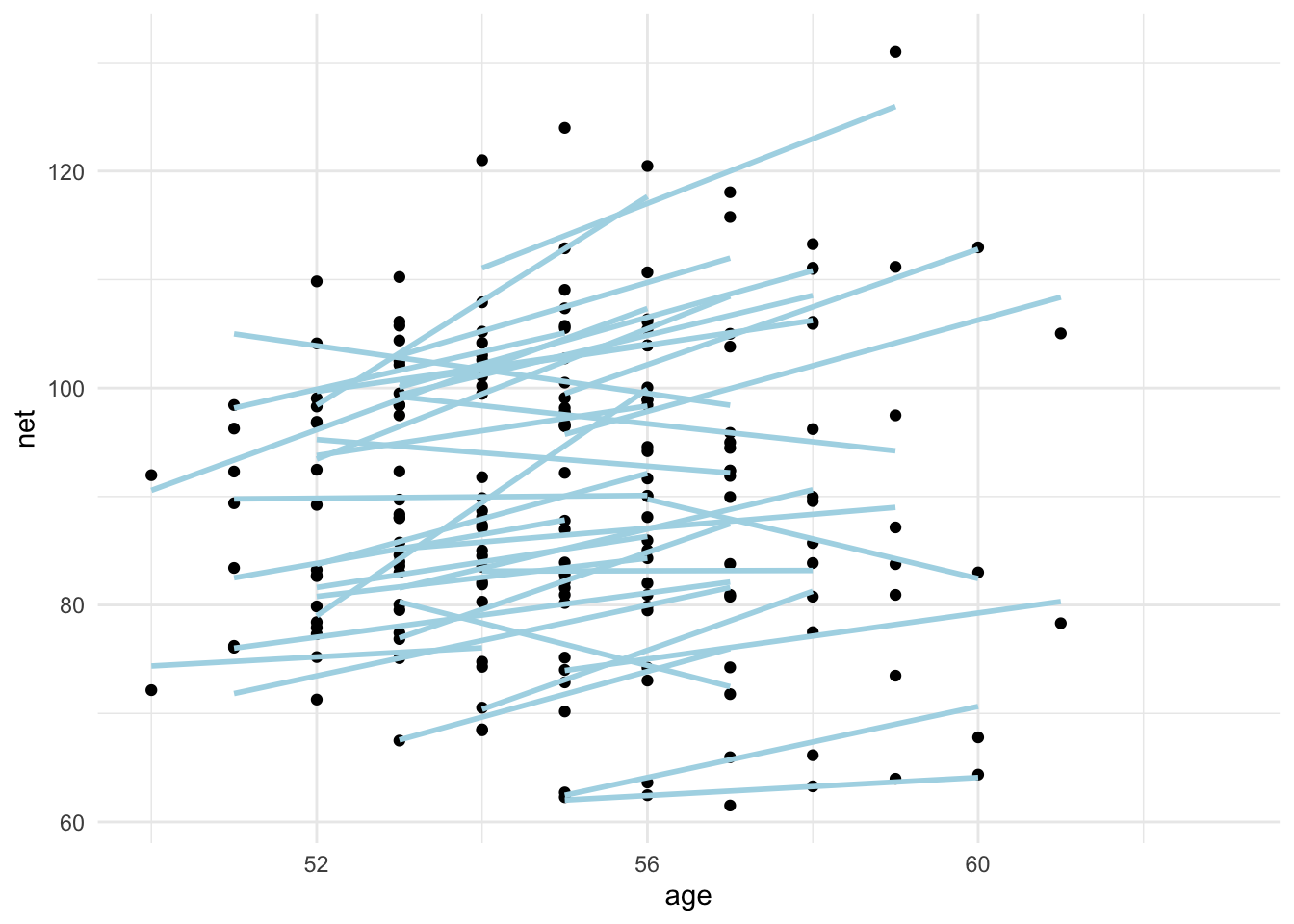
We see for most runners, the net time seems to be increasing with age. For some runners, that is not the case.
We would code this up as follows (this takes a long time to run):
nopool_model <- stan_glm(net ~ age + runner + age:runner,
  data = runners,
  family = gaussian,
  prior = normal(0, 2.5, autoscale = T),
  prior_intercept = normal(0, 2.5, autoscale = T),
  prior_aux = exponential(1, autoscale = T),
  refresh = 0
)
load("cached-simulations/nopool_model.rda")
broom.mixed::tidy(nopool_model, conf.int = T, conf.level = 0.9) %>%
filter(str_detect(term, "nter|age$|r[2-4]$"))broom.mixed::tidy(nopool_model, conf.int = T, conf.level = 0.9) %>%
filter(str_detect(term, "nter|age$|r[2-4]$"))- How do we interpret the
ageestimate of 1.02? - How do we interpret the
age:runner3estimate of -0.791? - What would you do if wanted to predict your own race time after you turn 50? Say you ran it 3 times at age 53, 55 and 57 with times 80, 81, and 80? What would you predict for your time at age 60?
Let’s look at a few plots:
filter(runners, runner %in% c(1, 3, 4, 5, 11, 33)) %>%
  ggplot(aes(age, net)) +
  geom_point() +
  geom_smooth(method = "lm", se = F) +
  facet_wrap(~runner)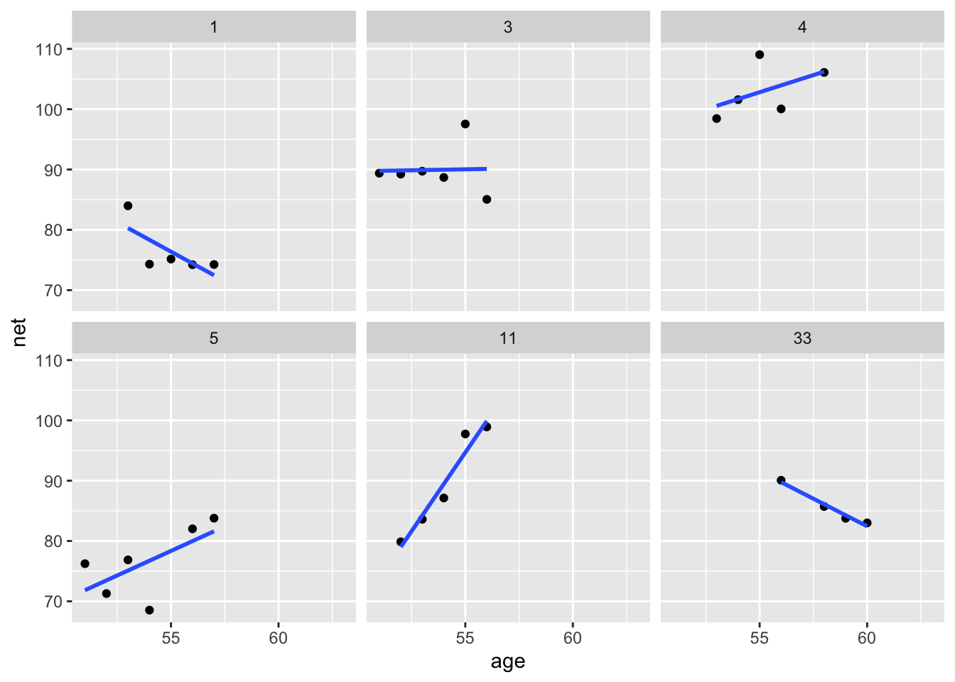
Consider a hierarchical model. In this case we imagine that each person will age differently. Some will improve, some will get worse, but the overall distribution of how people’s times change with age has its own distribution. We assume that the parent distribution is normal.
The following code is slow. You can load the output with the command ?
hier_model <- stan_glmer(net ~ age + (age | runner),
  data = runners,
  refresh = 0,
  adapt_delta = 0.99,
  iter = 10000
)bayesplot::mcmc_acf(hier_model, pars = "age")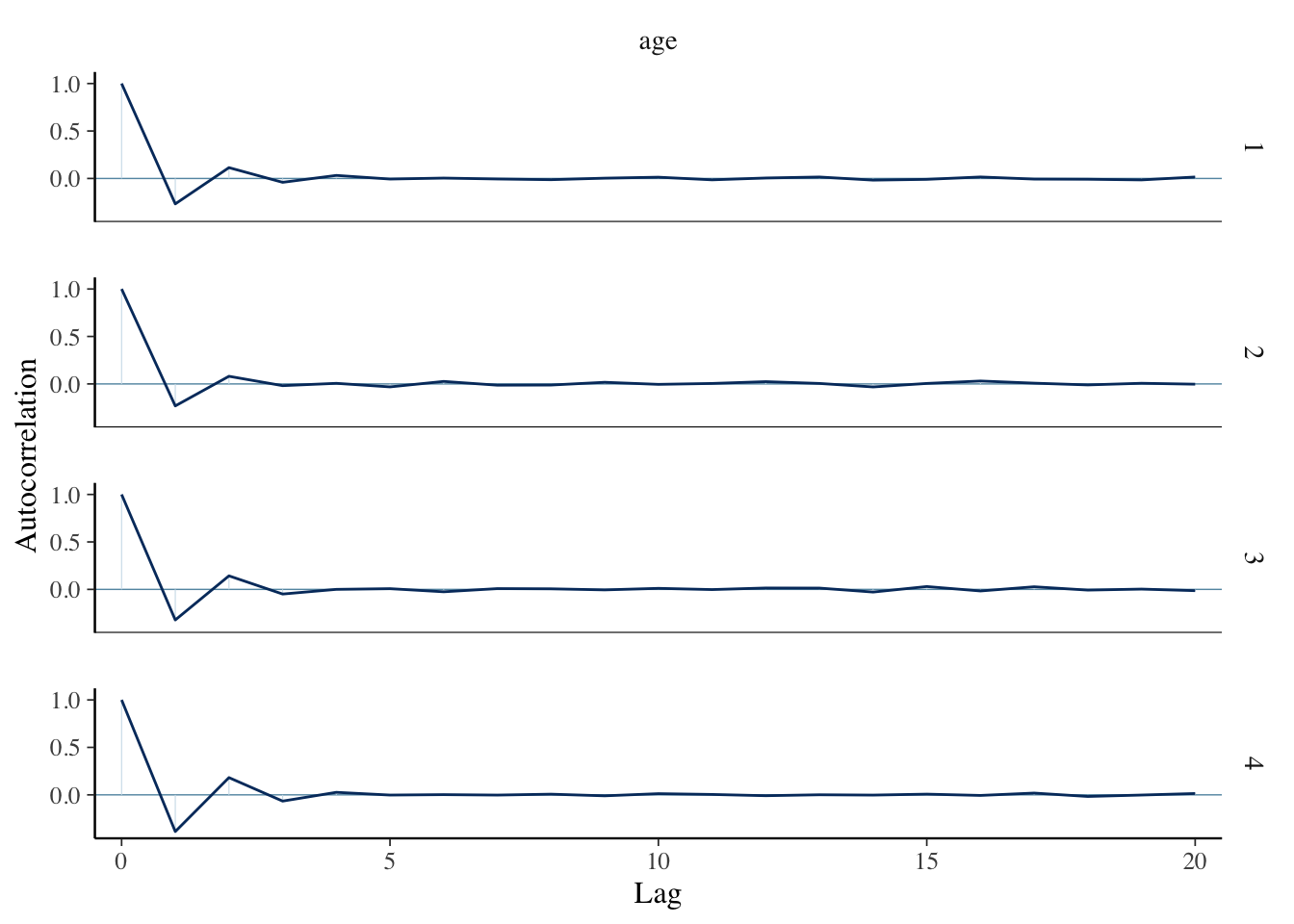
bayesplot::mcmc_dens_chains(hier_model, pars = "age")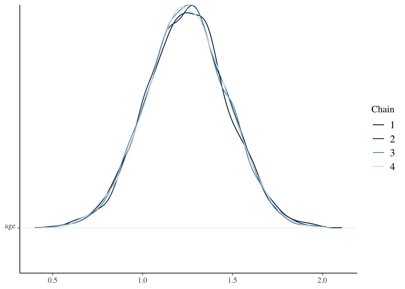
summary(hier_model)##
## Model Info:
## function: stan_glmer
## family: gaussian [identity]
## formula: net ~ age + (age | runner)
## algorithm: sampling
## sample: 20000 (posterior sample size)
## priors: see help('prior_summary')
## observations: 185
## groups: runner (36)
##
## Estimates:
## mean sd 10% 50% 90%
## (Intercept) 21.7 12.2 5.9 21.7 37.4
## age 1.2 0.2 1.0 1.2 1.5
## b[(Intercept) runner:1] 0.0 1.3 -0.8 0.0 0.8
## b[age runner:1] -0.2 0.1 -0.3 -0.2 -0.2
## b[(Intercept) runner:2] 0.0 1.1 -0.6 0.0 0.6
## b[age runner:2] -0.1 0.1 -0.2 -0.1 0.0
## b[(Intercept) runner:3] 0.0 1.0 -0.5 0.0 0.6
## b[age runner:3] 0.0 0.1 0.0 0.0 0.1
## b[(Intercept) runner:4] 0.0 1.3 -0.7 0.0 0.7
## b[age runner:4] 0.2 0.1 0.1 0.2 0.3
## b[(Intercept) runner:5] 0.0 1.2 -0.8 0.0 0.7
## b[age runner:5] -0.2 0.1 -0.3 -0.2 -0.1
## b[(Intercept) runner:6] 0.0 1.3 -0.8 0.0 0.8
## b[age runner:6] -0.3 0.1 -0.4 -0.3 -0.2
## b[(Intercept) runner:7] 0.0 1.3 -0.7 0.0 0.8
## b[age runner:7] 0.3 0.1 0.2 0.3 0.3
## b[(Intercept) runner:8] 0.0 1.3 -0.7 0.0 0.8
## b[age runner:8] 0.2 0.1 0.2 0.2 0.3
## b[(Intercept) runner:9] 0.0 1.2 -0.6 0.0 0.6
## b[age runner:9] 0.1 0.1 0.1 0.1 0.2
## b[(Intercept) runner:10] 0.0 1.7 -1.0 0.0 1.1
## b[age runner:10] 0.4 0.1 0.4 0.4 0.5
## b[(Intercept) runner:11] 0.0 1.1 -0.6 0.0 0.6
## b[age runner:11] 0.0 0.1 -0.1 0.0 0.1
## b[(Intercept) runner:12] 0.0 1.4 -0.9 0.0 0.8
## b[age runner:12] -0.3 0.1 -0.4 -0.3 -0.2
## b[(Intercept) runner:13] 0.0 1.2 -0.6 0.0 0.6
## b[age runner:13] -0.1 0.1 -0.2 -0.1 -0.1
## b[(Intercept) runner:14] 0.1 1.2 -0.6 0.0 0.7
## b[age runner:14] 0.1 0.1 0.0 0.1 0.2
## b[(Intercept) runner:15] 0.0 1.2 -0.6 0.0 0.7
## b[age runner:15] 0.1 0.1 0.0 0.1 0.2
## b[(Intercept) runner:16] 0.0 1.2 -0.6 0.0 0.6
## b[age runner:16] 0.1 0.1 0.0 0.1 0.2
## b[(Intercept) runner:17] 0.0 1.2 -0.7 0.0 0.7
## b[age runner:17] 0.2 0.1 0.1 0.2 0.3
## b[(Intercept) runner:18] 0.0 1.3 -0.7 0.0 0.8
## b[age runner:18] 0.2 0.1 0.1 0.2 0.3
## b[(Intercept) runner:19] 0.0 1.2 -0.6 0.0 0.6
## b[age runner:19] -0.1 0.1 -0.2 -0.1 -0.1
## b[(Intercept) runner:20] 0.0 1.5 -0.9 0.0 0.9
## b[age runner:20] 0.3 0.1 0.3 0.3 0.4
## b[(Intercept) runner:21] 0.0 1.1 -0.6 0.0 0.6
## b[age runner:21] -0.1 0.1 -0.2 -0.1 0.0
## b[(Intercept) runner:22] 0.0 1.1 -0.6 0.0 0.6
## b[age runner:22] 0.0 0.1 -0.1 0.0 0.1
## b[(Intercept) runner:23] 0.0 1.3 -0.7 0.0 0.8
## b[age runner:23] 0.2 0.1 0.2 0.2 0.3
## b[(Intercept) runner:24] 0.0 1.2 -0.7 0.0 0.7
## b[age runner:24] 0.2 0.1 0.1 0.2 0.3
## b[(Intercept) runner:25] 0.1 1.2 -0.6 0.0 0.8
## b[age runner:25] 0.2 0.1 0.1 0.2 0.3
## b[(Intercept) runner:26] 0.0 1.1 -0.6 0.0 0.6
## b[age runner:26] 0.0 0.1 -0.1 0.0 0.0
## b[(Intercept) runner:27] 0.0 1.3 -0.7 0.0 0.7
## b[age runner:27] 0.2 0.1 0.1 0.2 0.3
## b[(Intercept) runner:28] 0.0 1.2 -0.7 0.0 0.7
## b[age runner:28] -0.2 0.1 -0.3 -0.2 -0.1
## b[(Intercept) runner:29] 0.0 1.8 -1.2 0.0 1.1
## b[age runner:29] -0.5 0.1 -0.6 -0.5 -0.4
## b[(Intercept) runner:30] 0.0 1.7 -1.1 0.0 1.0
## b[age runner:30] -0.5 0.1 -0.5 -0.5 -0.4
## b[(Intercept) runner:31] 0.0 1.1 -0.6 0.0 0.6
## b[age runner:31] -0.1 0.1 -0.2 -0.1 0.0
## b[(Intercept) runner:32] 0.0 1.2 -0.7 0.0 0.7
## b[age runner:32] -0.2 0.1 -0.3 -0.2 -0.1
## b[(Intercept) runner:33] 0.0 1.2 -0.6 0.0 0.6
## b[age runner:33] -0.1 0.1 -0.2 -0.1 -0.1
## b[(Intercept) runner:34] 0.0 1.3 -0.8 0.0 0.7
## b[age runner:34] -0.3 0.1 -0.3 -0.3 -0.2
## b[(Intercept) runner:35] 0.0 1.1 -0.6 0.0 0.6
## b[age runner:35] -0.1 0.1 -0.2 -0.1 0.0
## b[(Intercept) runner:36] 0.0 1.3 -0.8 0.0 0.9
## b[age runner:36] 0.3 0.1 0.2 0.3 0.4
## sigma 5.2 0.3 4.8 5.2 5.6
## Sigma[runner:(Intercept),(Intercept)] 1.6 8.6 0.0 0.1 2.4
## Sigma[runner:age,(Intercept)] 0.0 0.2 -0.1 0.0 0.1
## Sigma[runner:age,age] 0.1 0.0 0.0 0.1 0.1
##
## Fit Diagnostics:
## mean sd 10% 50% 90%
## mean_PPD 89.9 0.5 89.2 89.9 90.6
##
## The mean_ppd is the sample average posterior predictive distribution of the outcome variable (for details see help('summary.stanreg')).
##
## MCMC diagnostics
## mcse Rhat n_eff
## (Intercept) 0.1 1.0 38440
## age 0.0 1.0 34179
## b[(Intercept) runner:1] 0.0 1.0 4422
## b[age runner:1] 0.0 1.0 12966
## b[(Intercept) runner:2] 0.0 1.0 14095
## b[age runner:2] 0.0 1.0 16792
## b[(Intercept) runner:3] 0.0 1.0 18823
## b[age runner:3] 0.0 1.0 15106
## b[(Intercept) runner:4] 0.0 1.0 5687
## b[age runner:4] 0.0 1.0 13704
## b[(Intercept) runner:5] 0.0 1.0 4926
## b[age runner:5] 0.0 1.0 12662
## b[(Intercept) runner:6] 0.0 1.0 3775
## b[age runner:6] 0.0 1.0 13318
## b[(Intercept) runner:7] 0.0 1.0 4058
## b[age runner:7] 0.0 1.0 12928
## b[(Intercept) runner:8] 0.0 1.0 4051
## b[age runner:8] 0.0 1.0 12227
## b[(Intercept) runner:9] 0.0 1.0 11344
## b[age runner:9] 0.0 1.0 15635
## b[(Intercept) runner:10] 0.0 1.0 2574
## b[age runner:10] 0.0 1.0 8295
## b[(Intercept) runner:11] 0.0 1.0 16106
## b[age runner:11] 0.0 1.0 16221
## b[(Intercept) runner:12] 0.0 1.0 3307
## b[age runner:12] 0.0 1.0 11035
## b[(Intercept) runner:13] 0.0 1.0 8747
## b[age runner:13] 0.0 1.0 15488
## b[(Intercept) runner:14] 0.0 1.0 14031
## b[age runner:14] 0.0 1.0 15084
## b[(Intercept) runner:15] 0.0 1.0 9370
## b[age runner:15] 0.0 1.0 15442
## b[(Intercept) runner:16] 0.0 1.0 14747
## b[age runner:16] 0.0 1.0 16193
## b[(Intercept) runner:17] 0.0 1.0 5021
## b[age runner:17] 0.0 1.0 16100
## b[(Intercept) runner:18] 0.0 1.0 5354
## b[age runner:18] 0.0 1.0 14331
## b[(Intercept) runner:19] 0.0 1.0 8684
## b[age runner:19] 0.0 1.0 14091
## b[(Intercept) runner:20] 0.0 1.0 2917
## b[age runner:20] 0.0 1.0 10790
## b[(Intercept) runner:21] 0.0 1.0 11426
## b[age runner:21] 0.0 1.0 15247
## b[(Intercept) runner:22] 0.0 1.0 16501
## b[age runner:22] 0.0 1.0 16140
## b[(Intercept) runner:23] 0.0 1.0 4973
## b[age runner:23] 0.0 1.0 13020
## b[(Intercept) runner:24] 0.0 1.0 4377
## b[age runner:24] 0.0 1.0 13191
## b[(Intercept) runner:25] 0.0 1.0 5920
## b[age runner:25] 0.0 1.0 14786
## b[(Intercept) runner:26] 0.0 1.0 15910
## b[age runner:26] 0.0 1.0 15682
## b[(Intercept) runner:27] 0.0 1.0 5620
## b[age runner:27] 0.0 1.0 13400
## b[(Intercept) runner:28] 0.0 1.0 6006
## b[age runner:28] 0.0 1.0 13952
## b[(Intercept) runner:29] 0.0 1.0 2234
## b[age runner:29] 0.0 1.0 6839
## b[(Intercept) runner:30] 0.0 1.0 2465
## b[age runner:30] 0.0 1.0 8120
## b[(Intercept) runner:31] 0.0 1.0 9456
## b[age runner:31] 0.0 1.0 14388
## b[(Intercept) runner:32] 0.0 1.0 6710
## b[age runner:32] 0.0 1.0 14376
## b[(Intercept) runner:33] 0.0 1.0 8677
## b[age runner:33] 0.0 1.0 14961
## b[(Intercept) runner:34] 0.0 1.0 4143
## b[age runner:34] 0.0 1.0 12502
## b[(Intercept) runner:35] 0.0 1.0 13316
## b[age runner:35] 0.0 1.0 15012
## b[(Intercept) runner:36] 0.0 1.0 3253
## b[age runner:36] 0.0 1.0 13439
## sigma 0.0 1.0 21519
## Sigma[runner:(Intercept),(Intercept)] 0.1 1.0 11401
## Sigma[runner:age,(Intercept)] 0.0 1.0 2485
## Sigma[runner:age,age] 0.0 1.0 6150
## mean_PPD 0.0 1.0 20150
## log-posterior 0.1 1.0 4866
##
## For each parameter, mcse is Monte Carlo standard error, n_eff is a crude measure of effective sample size, and Rhat is the potential scale reduction factor on split chains (at convergence Rhat=1).broom.mixed::tidy(hier_model, conf.int = T)## # A tibble: 2 × 5
## term estimate std.error conf.low conf.high
## <chr> <dbl> <dbl> <dbl> <dbl>
## 1 (Intercept) 21.7 12.1 1.43 41.7
## 2 age 1.25 0.223 0.876 1.62library(tidybayes)
draws <- tidybayes::spread_draws(hier_model, `[\\(a-z].*`, regex = T, ndraws = 100) %>%
janitor::clean_names()Let’s plot 100 or so draws of lines of best fit for runner 2 on the scatterplot of runner 2’s times.
runners %>%
  filter(runner == "2") %>%
  ggplot(aes(age, net)) +
  geom_point() +
  geom_abline(
    intercept = draws$intercept + draws$b_intercept_runner_2,
    slope = draws$age + draws$b_age_runner_2
  ) +
  scale_y_continuous(limits = c(70, 100))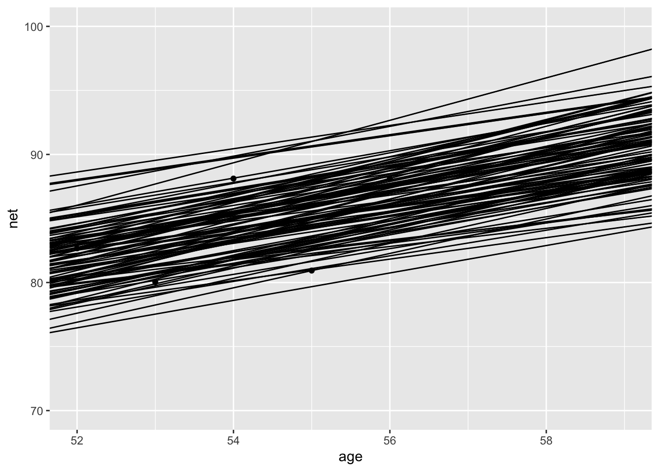
ggplot(runners, aes(age, net)) +
  geom_point() +
  geom_abline(intercept = draws$intercept, slope = draws$age, alpha = 0.3) +
  geom_smooth(method = "lm", se = F, color = "red")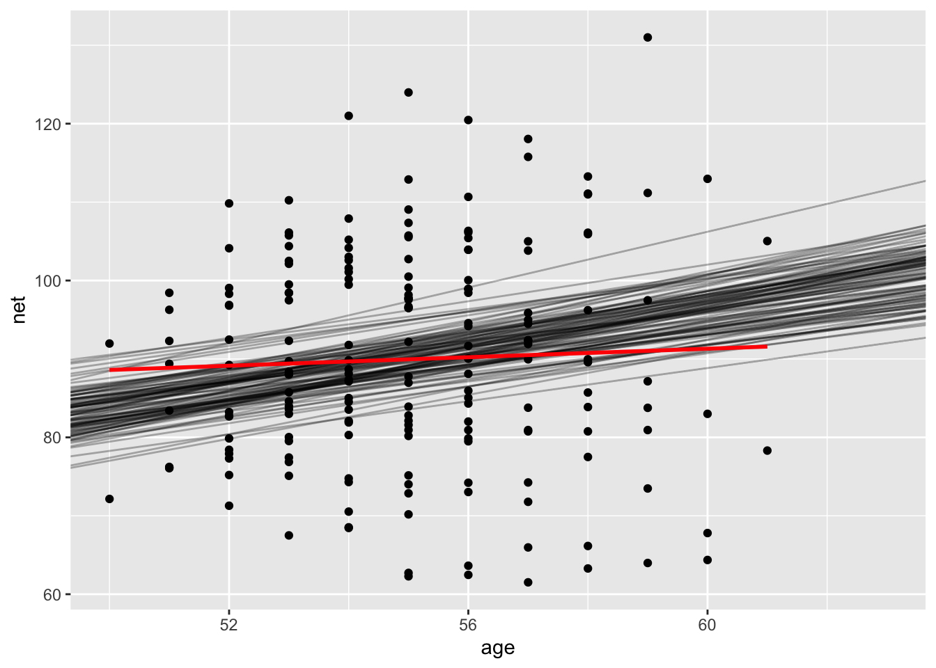
Which of the the two lines is “more appropriate” to use as our model of