Chapter 6 Logistic Regression
In this short chapter, we talk about logistic regression. We assume that we have data such that the response \(Y\) is classified as either success or failure. We assume that we have one or more predictors, which we want to use to estimate the probability of success \(p\), which will depend on the predictors.
Odds are something that isn’t always talked about in probability class. If the probability of an event \(A\) is \(p\), then the odds of \(A\) are defined to be \(\frac{p}{1- p}\). This is often written in the form 3:1 and read “three to one (in favor of \(A\)).” What this means in practice is that, on average, we6 expect that \(A\) will happen 3 times for every 1 time it does not happen. In other words, the probability of \(A\) is 3/4.
If you have the odds \(O\) (in favor) of an event \(A\), and you want the probability, you solve \(O = \frac{p}{1-p}\) for \(p\), so \(p = \frac{O}{1 + O}\). For example, if the odds are 1:4 in favor of \(A\), you would get \(p = \frac{.25}{1.25} = 1/5\).
We assume \(Y|_{X = x, \beta_0, \beta_1} \sim \mathrm{Binom}(1, p)\), where the log odds \(\log \frac{p}{1-p} = \beta_0 + \beta_1 x\). Let’s look at an example.
malaria <- fosdata::malaria
ggplot(malaria, aes(sporozoite, malaria, color = antibody)) +
  geom_jitter(height = 0, width = .4, alpha = .3)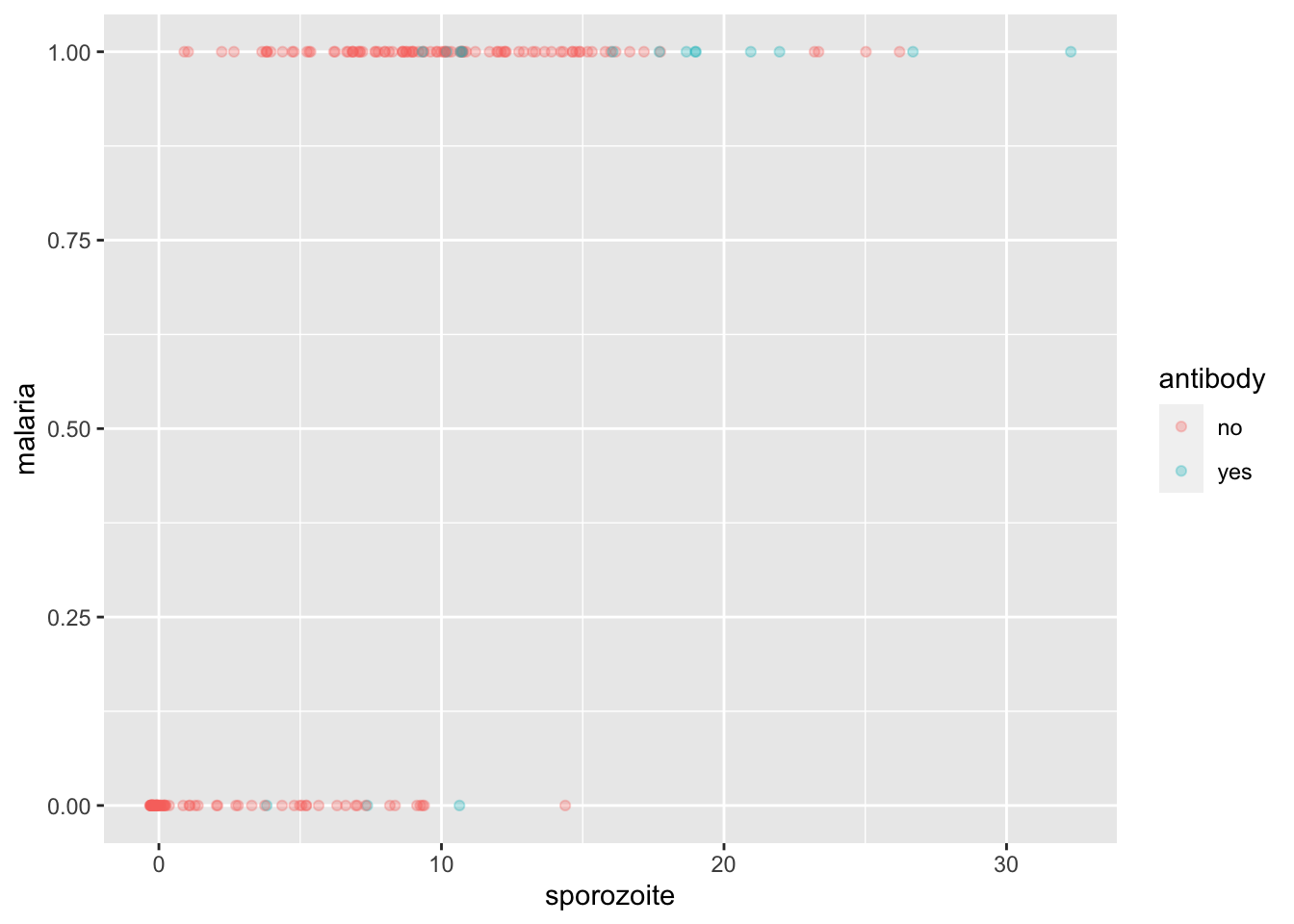
We build our model:
malaria_model <- rstanarm::stan_glm(malaria ~ sporozoite,
  data = malaria,
  family = binomial,
  refresh = 0
)

broom.mixed::tidy(malaria_model)
## # A tibble: 2 × 3
## term estimate std.error
## <chr> <dbl> <dbl>
## 1 (Intercept) -2.46 0.431
## 2 sporozoite 0.457 0.0653We get point estimates of \(\beta_0 = -2.46\) and \(\beta_1 = .458\). Let’s think about what these mean! When the predictor is equal to 0 (that is, when there are no sporozoites), the log odds of the mouse getting malaria is \(\log \frac {p}{1-p} = -2.46\). The log-odds can be hard to interpret until you get used to them, so we rewrite in terms of \(p\). Solving for \(p\), we get \(p = \frac{e^{-2.46}}{1 + e^{-2.46}} = 0.07871034\). This can also be done with
rstanarm::invlogit(-2.46)## [1] 0.07871034The bottom line is that our model assigns an 8 percent probability to getting malaria if the mosquito that bit you has no sporozoites, which I think cannot be correct, but which still may be useful.
What about the interpretation of \(\beta_1\)? Well, for each unit increase in the predictor, the log odds increases by \(\beta_1\). Let’s write \(O_x\) for the log odds when \(X = x\). So, \(O_{x + k} = k \beta_1 + O_x\). Exponentiating both sides we get that the odds when \(X = x + k\) are \(e^{k \beta_1}\) times the odds when \(X = x\).
Let’s look at some plots and see if we can estimate some parameter values.
ggplot(malaria, aes(sporozoite, malaria)) +
  geom_jitter(height = 0, width = .2, alpha = .3) +
  geom_function(fun = function(x) rstanarm::invlogit(-2.46 + .458 * x))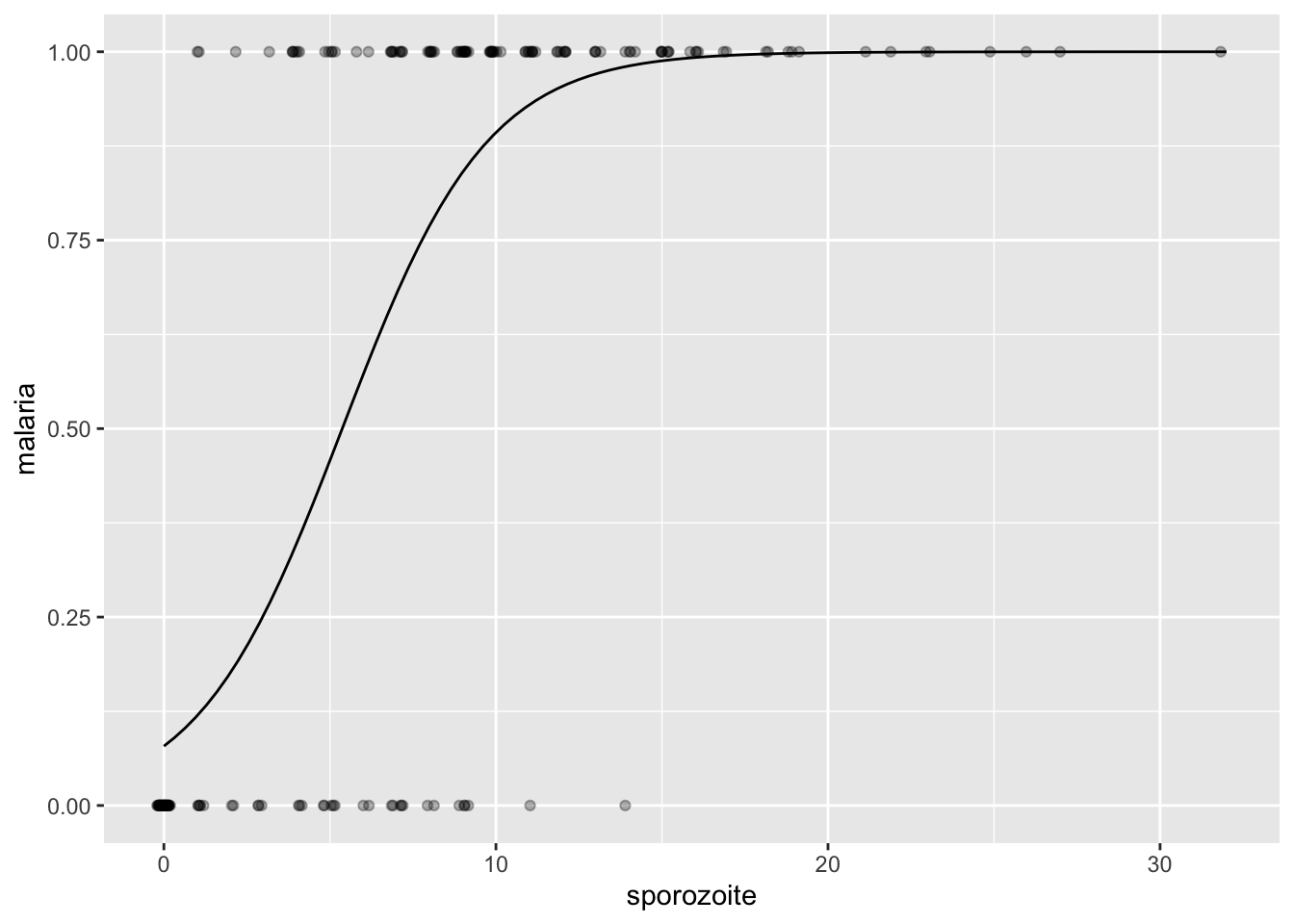
For \(\beta_0\), we have the odds of getting malaria when \(X = 0\) are \(e^{\beta_0}\). We had that about 1 in 24 people got malaria when bitten by a mosquito with 1 or fewer sporozoites, so the odds are also about 1 to 24 (they are 1 to 23). So, \(e^{\beta_0} \approx 1/23\), so \(\beta_0 \approx -3.14\).
malaria %>%
  filter(sporozoite <= 1) %>%
  summarize(
    p = mean(malaria),
    o = 1 / p
  )
## # A tibble: 1 × 2
## p o
## <dbl> <dbl>
## 1 0.0417 24How could we have estimated \(\beta_1\)? Let’s estimate the odds of getting malaria when there are about 5 sporozoites versus the odds when there are about 10.
malaria %>%
  filter(abs(sporozoite - 5) < 2 | abs(sporozoite - 10) < 2) %>%
  group_by(cut(sporozoite, 2)) %>%
  summarize(
    p = mean(malaria),
    o = p / (1 - p)
  )
## # A tibble: 2 × 3
## `cut(sporozoite, 2)` p o
## <fct> <dbl> <dbl>
## 1 (3.99,7.5] 0.565 1.3
## 2 (7.5,11] 0.865 6.4Therefore, the odds of getting malaria increased from 1.3:1 to 6.4:1, and \(e^{5 \beta_1} \approx 6.4/1.3 \approx 5\), so \(\beta_1 \approx \frac 15\log 5 \approx .322.\) The true estimate from above was .457, which is pretty close to our rough guide here.
Let’s check some posterior plots. We might be interested in the proportion of time our model predicts malaria versus the proportion of times that malaria actually occurs.
proportion_malaria <- function(x) {
  mean(x == 1)
}
rstanarm::pp_check(malaria_model,
  plotfun = "stat",
  stat = "proportion_malaria",
  binwidth = .016
) +
  xlab("probability of malaria")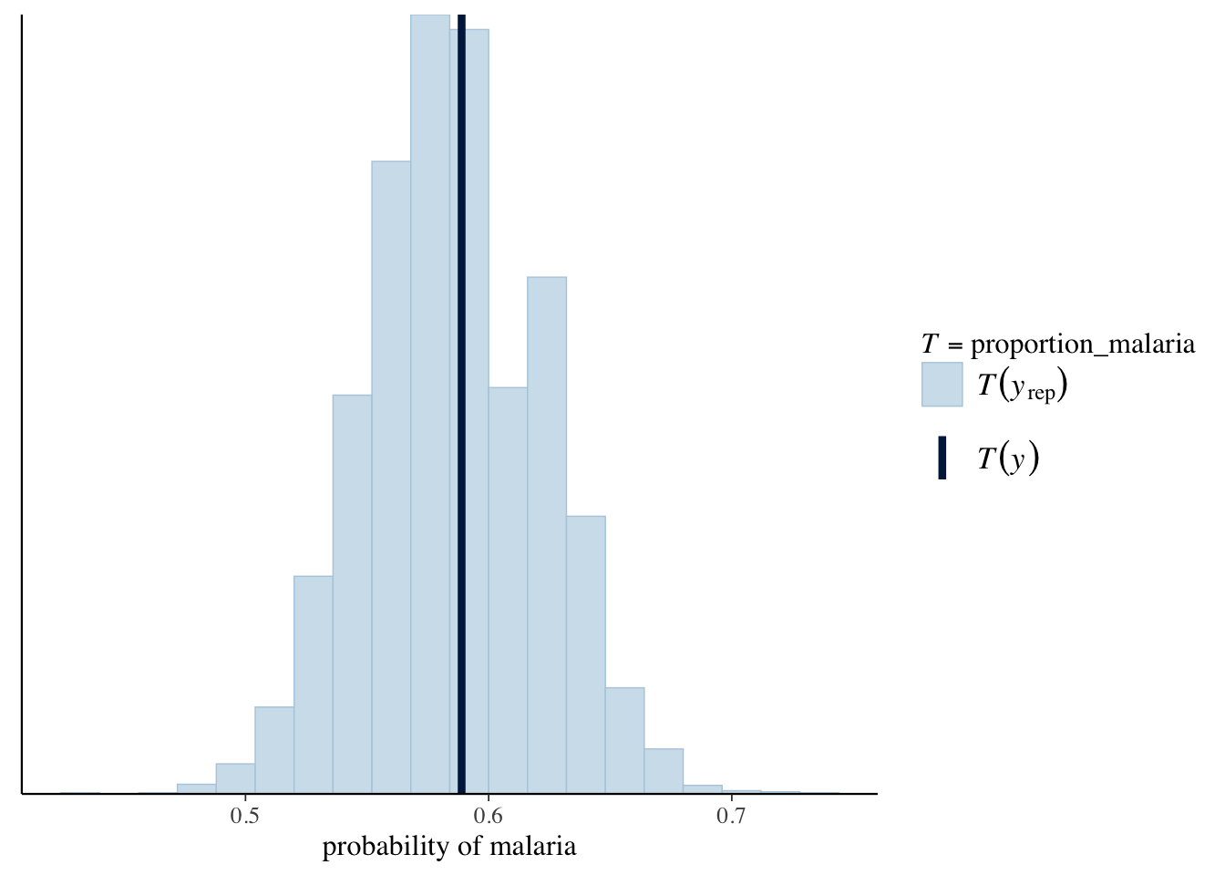
malaria$id <- 1:180
tidybayes::add_predicted_draws(newdata = malaria, object = malaria_model, ndraws = 1000) %>%
  group_by(.draw) %>%
  summarize(p = mean(.prediction)) %>%
  ggplot(aes(x = p)) +
  geom_histogram(bins = 17, fill = "lightblue", color = "gray") +
  theme_minimal() +
  geom_vline(xintercept = mean(malaria$malaria))
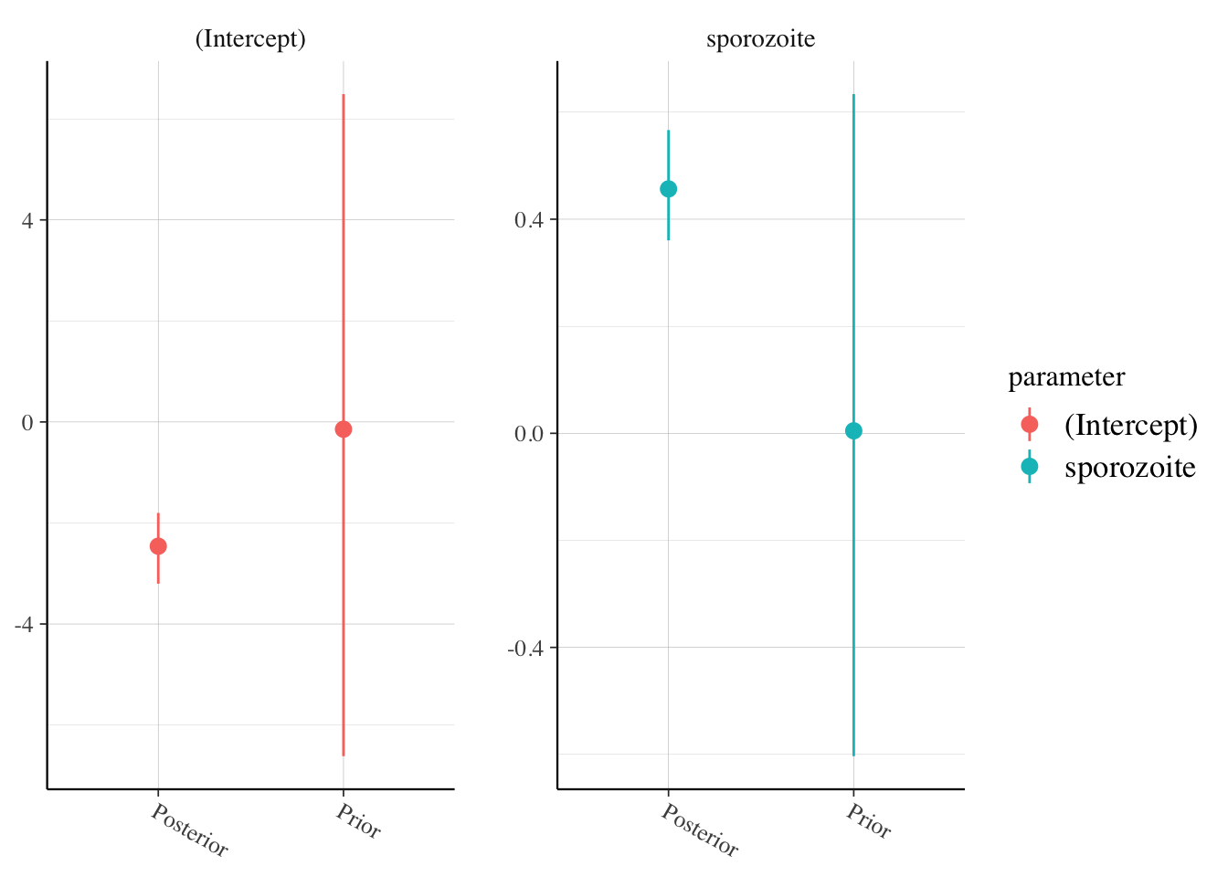
This looks pretty good. We should also check posterior versus priors.
rstanarm::posterior_vs_prior(malaria_model,
  facet_args = list(scales = "free"),
  group_by_parameter = T
)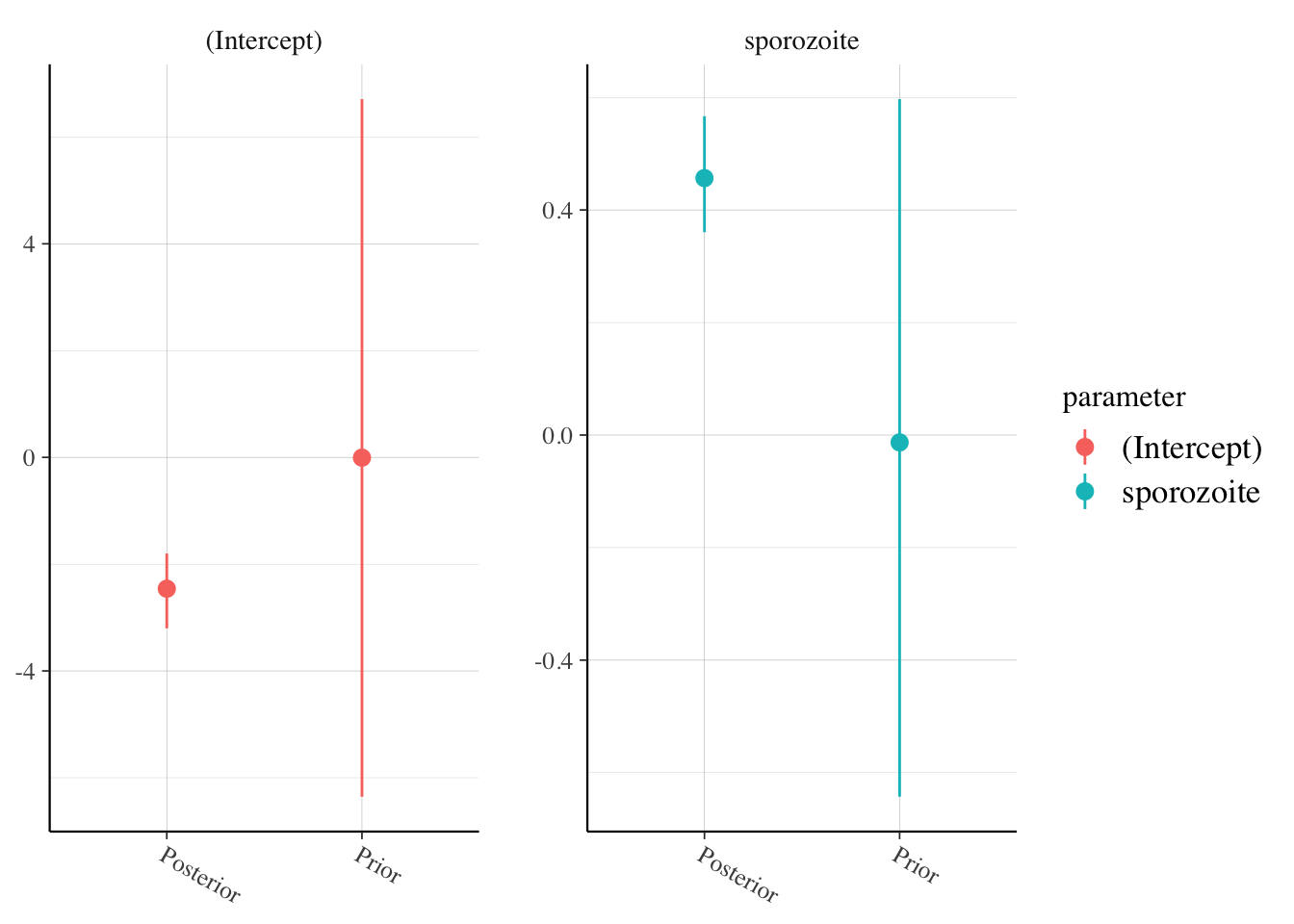
Both look OK.
Find reasonable weakly informative priors for \(\beta_0\) and \(\beta_1\).
We contine along the line of reasoning that we used above. One issue is that rstanarm uses the centered predictors for the prior of the intercept. Since the mean number of sporozoite is 8, that means that \(\beta_{0c}\) satisfies \(\beta_{0c} \approx \log {p}{1-p}\), the log odds of getting malaria when bitten by a mosquito with 8 sporozoites. Let’s figure that out.
malaria %>%
  filter(sporozoite > 5 & sporozoite < 11) %>%
  summarize(
    p = mean(malaria),
    logodds = log(p / (1 - p))
  )
## # A tibble: 1 × 2
## p logodds
## <dbl> <dbl>
## 1 0.759 1.15Therefore, \(\beta_{0c} \approx 1.15\). It seems reasonable to say the true probability of getting malaria with 8 sporozoites is between .05 and .99, which leads to values of \(\beta_{0c}\) between -3 and 4.5. So, perhaps \(\beta_{0c} \sim N(1, 3.5)\) would be a good weak prior.
log(.05 / (1 - .05))## [1] -2.944439log(.99 / (1 - .99))## [1] 4.59512We want to find bounds for \(\beta_0\) which indicate what we think is plausible. Of course, in this case, it might be reasonable to set the probability of getting malaria equal to 0 if there are really no sporozoites in the mosquito, but we want the probability if no sporozoites were measured in the sample. We found our point estimate for \(\beta_0\) to be about -3.14, which corresponds to a 4 percent chance of getting malaria. A plausible bound could be a probability of getting malaria between .01 and .2. This corresponds to \(\beta_0\) between \(-4.6\) and \(-1.4\):
c(rstanarm::logit(.01), rstanarm::logit(.2))## [1] -4.595120 -1.386294So, perhaps a reasonable weakly informative prior for \(\beta_0\) would be \(N(-3, 1.6)\).
Turning to \(\beta_1\), it is perhaps reasonable to assume that the probability of getting malaria with 5 sporozoites is at least .1 and for 10 sporozoites it is at most .99. We also assume that \(\beta_1\) is most likely positive. This would lead to \(\beta_1\) estimates between 0 and 1.4, so perhaps a good prior would be \(N(.7, .7)\).
log(1000) / 5## [1] 1.381551Let’s test it out:
library(rstanarm)
malaria_model_prior <- stan_glm(malaria ~ sporozoite,
  data = malaria,
  family = binomial,
  refresh = 0,
  prior_intercept = normal(1, 3.5, autoscale = F),
  prior = normal(0.7, 0.7, autoscale = F)
)
prior_summary(malaria_model_prior)
## Priors for model 'malaria_model_prior'
## ------
## Intercept (after predictors centered)
## ~ normal(location = 1, scale = 3.5)
##
## Coefficients
## ~ normal(location = 0.7, scale = 0.7)
## ------
## See help('prior_summary.stanreg') for more detailsbroom.mixed::tidy(malaria_model_prior)## # A tibble: 2 × 3
## term estimate std.error
## <chr> <dbl> <dbl>
## 1 (Intercept) -2.56 0.437
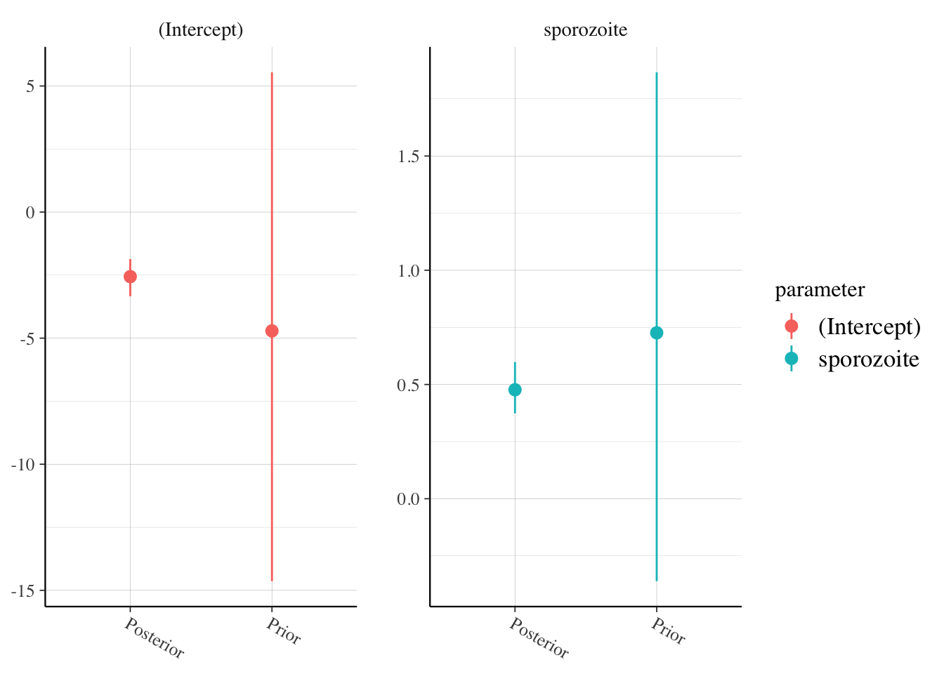
## 2 sporozoite 0.477 0.0648posterior_vs_prior(malaria_model_prior,
facet_args = list(scales = "free"),
group_by_parameter = T
)
posterior_vs_prior(malaria_model,
  facet_args = list(scales = "free"),
  group_by_parameter = T
)
prior_summary(malaria_model)## Priors for model 'malaria_model'
## ------
## Intercept (after predictors centered)
## ~ normal(location = 0, scale = 2.5)
##
## Coefficients
## Specified prior:
## ~ normal(location = 0, scale = 2.5)
## Adjusted prior:
## ~ normal(location = 0, scale = 0.38)
## ------
## See help('prior_summary.stanreg') for more detailsThe Bayesian would not necessarily agree with this interpretation.↩︎